Multiple Regression Model

workflowr

• Summary
• Checks
• Past versions

Last updated: 2019-11-15

Checks: 7 0

Knit directory: STA_463_563_Fall2019/

This reproducible R Markdown analysis was created with workflowr (version 1.4.0). The Checks tab describes the reproducibility checks that were applied when the results were created. The Past versions tab lists the development history.

---

R Markdown file: up-to-date

Great! Since the R Markdown file has been committed to the Git repository, you know the exact version of the code that produced these results.

Environment: empty

Great job! The global environment was empty. Objects defined in the global environment can affect the analysis in your R Markdown file in unknown ways. For reproduciblity it’s best to always run the code in an empty environment.

Seed: set.seed(20190905)

The command set.seed(20190905) was run prior to running the code in the R Markdown file. Setting a seed ensures that any results that rely on randomness, e.g. subsampling or permutations, are reproducible.

Session information: recorded

Great job! Recording the operating system, R version, and package versions is critical for reproducibility.

Cache: none

Nice! There were no cached chunks for this analysis, so you can be confident that you successfully produced the results during this run.

File paths: relative

Great job! Using relative paths to the files within your workflowr project makes it easier to run your code on other machines.

Repository version: d3d57a4

Great! You are using Git for version control. Tracking code development and connecting the code version to the results is critical for reproducibility. The version displayed above was the version of the Git repository at the time these results were generated.

Note that you need to be careful to ensure that all relevant files for the analysis have been committed to Git prior to generating the results (you can use wflow_publish or wflow_git_commit). workflowr only checks the R Markdown file, but you know if there are other scripts or data files that it depends on. Below is the status of the Git repository when the results were generated:

Ignored files:
    Ignored:    .DS_Store
    Ignored:    .Rhistory
    Ignored:    .Rproj.user/
    Ignored:    analysis/.DS_Store

Note that any generated files, e.g. HTML, png, CSS, etc., are not included in this status report because it is ok for generated content to have uncommitted changes.

---

These are the previous versions of the R Markdown and HTML files. If you’ve configured a remote Git repository (see ?wflow_git_remote), click on the hyperlinks in the table below to view them.

File	Version	Author	Date	Message
Rmd	d3d57a4	dleelab	2019-11-15	added
html	2f6bbe8	dleelab	2019-11-15	created
Rmd	2bac0d3	dleelab	2019-11-15	created

---

Fit model with transformed predictor/response

Plastic hardness data, fit \(Y=\beta_0+\beta_1X+\epsilon\).

plastic=read.table("http://users.stat.ufl.edu/~rrandles/sta4210/Rclassnotes/data/textdatasets/KutnerData/Chapter%20%201%20Data%20Sets/CH01PR22.txt")
colnames(plastic)=c("Y","X")
lm(Y~X,data=plastic)

Call:
lm(formula = Y ~ X, data = plastic)

Coefficients:
(Intercept)            X  
    168.600        2.034  

lm(Y~X^2,data=plastic)

Call:
lm(formula = Y ~ X^2, data = plastic)

Coefficients:
(Intercept)            X  
    168.600        2.034  

What’s wrong with the above result?

Solutions:

Y2=(plastic$Y)^2
X2=(plastic$X)^2
lm(Y~X2,data=plastic)

Call:
lm(formula = Y ~ X2, data = plastic)

Coefficients:
(Intercept)           X2  
  194.88253      0.03551  

lm(Y~I(X^2),data=plastic)

Call:
lm(formula = Y ~ I(X^2), data = plastic)

Coefficients:
(Intercept)       I(X^2)  
  194.88253      0.03551  

Multiple Regression Fit (Lecture 13)

1. Data: The Prestige data frame is the Prestige of Canadian Occupations. It has 102 rows and 6 columns. The observations are occupations. First of all, we remove all observations that have missing values for varaible ``type’’.

#install.packages("car")
library(car)

Loading required package: carData

#?Prestige
mydata=Prestige[!is.na(Prestige$type), ]#remove the observations with missing values for "type"
unique(mydata$type)

[1] prof bc   wc  
Levels: bc prof wc

To have an idea about the predictor variable and the response, we can view the enhanced scatterplot.

scatterplot(income~education|type, data=mydata,ylab="Income",
            xlab="Education",main="Income vs Education")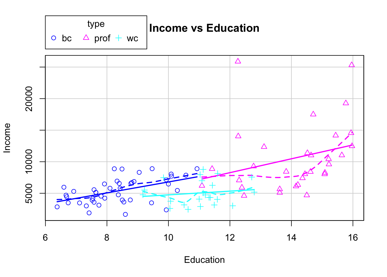

Past versions of unnamed-chunk-4-1.png

Version	Author	Date
2f6bbe8	dleelab	2019-11-15

Based on the plot, maybe there’s linear relationsihp between education and income. It seems the intercept of bc and prof are similar, different from that of the wc. We also want know whether the slope of the three groups are different (whether interaction term is necessary).

Alternative method using the ggplot:

library(ggplot2)
ggplot(data=mydata, aes(x=education, y=income)) + 
  geom_point(aes(colour = factor(type))) +
  geom_smooth(aes(colour = factor(type)))

`geom_smooth()` using method = 'loess' and formula 'y ~ x'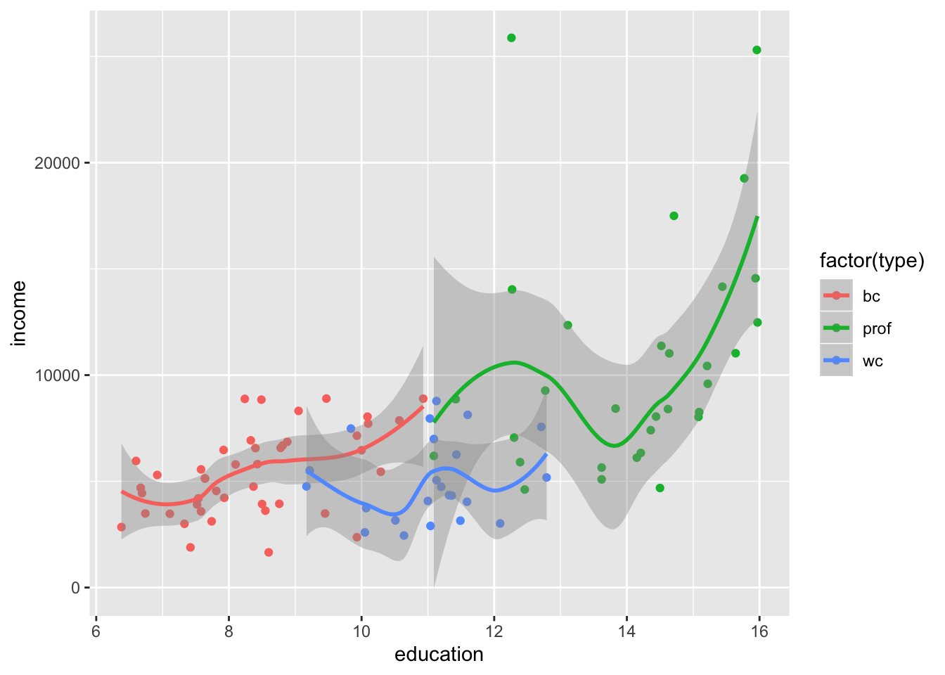

Past versions of unnamed-chunk-5-1.png

Version	Author	Date
2f6bbe8	dleelab	2019-11-15

2. Generate the design matrix

X=model.matrix(~type,data=mydata)
#X
Y=as.matrix(mydata$income)
solve(t(X)%*%X)%*%t(X)%*%Y

                [,1]
(Intercept) 5374.136
typeprof    5185.315
typewc      -321.832

lm(income~type,data=mydata)#automatically, bc is the reference group.

Call:
lm(formula = income ~ type, data = mydata)

Coefficients:
(Intercept)     typeprof       typewc  
     5374.1       5185.3       -321.8  

3. Mix continuous and categorical variable.

(1) Use income as response, education and type as predictor.

X=model.matrix(~education+type,data=mydata)
#X
Y=as.matrix(mydata$income)
solve(t(X)%*%X)%*%t(X)%*%Y

                  [,1]
(Intercept) -2048.2080
education     887.9126
typeprof      102.1260
typewc      -2685.8293

lm(income~education+type,data=mydata)

Call:
lm(formula = income ~ education + type, data = mydata)

Coefficients:
(Intercept)    education     typeprof       typewc  
    -2048.2        887.9        102.1      -2685.8  

#If the data is in letters, R recognize it as a categorical factor.

(2) If you don’t like bc be reference group, change it to wc.

new=relevel(mydata$type,ref="wc")
X=model.matrix(~education+new,data=mydata)
Y=as.matrix(mydata$income)
solve(t(X)%*%X)%*%t(X)%*%Y

                  [,1]
(Intercept) -4734.0372
education     887.9126
newbc        2685.8293
newprof      2787.9553

lm(income~education+new,data=mydata)

Call:
lm(formula = income ~ education + new, data = mydata)

Coefficients:
(Intercept)    education        newbc      newprof  
    -4734.0        887.9       2685.8       2788.0  

(3) Like constructing a linear regression model, you may also include interaction terms

X=model.matrix(~education+type+education*type,data=mydata)
Y=as.matrix(mydata$income)
solve(t(X)%*%X)%*%t(X)%*%Y

                         [,1]
(Intercept)        -1865.0362
education            866.0004
typeprof           -3068.3645
typewc              3646.5441
education:typeprof   234.0166
education:typewc    -569.2417

lm(income~education+type+education*type,data=mydata)

Call:
lm(formula = income ~ education + type + education * type, data = mydata)

Coefficients:
       (Intercept)           education            typeprof  
           -1865.0               866.0             -3068.4  
            typewc  education:typeprof    education:typewc  
            3646.5               234.0              -569.2  

4. What if you want a categorical variable, but it’s coded in 1,2,3, etc.

(1) Directly use it, R will recognize it as numeric variable.

mydata2=cbind(mydata,c(rep(1,40),rep(2,38),rep(3,20)))
colnames(mydata2)[7]=c("group")
#mydata2
lm(income~group,data=mydata2)

Call:
lm(formula = income ~ group, data = mydata2)

Coefficients:
(Intercept)        group  
       9889        -1643  

(2) We can manually let R know it’s a categorical variable.

mydata2$group=factor(mydata2$group)
lm(income~group,data=mydata2)

Call:
lm(formula = income ~ group, data = mydata2)

Coefficients:
(Intercept)       group2       group3  
       8891        -3643        -2641  

#alternative way
groupf=factor(mydata2$group)
lm(income~groupf,data=mydata2)

Call:
lm(formula = income ~ groupf, data = mydata2)

Coefficients:
(Intercept)      groupf2      groupf3  
       8891        -3643        -2641  

#alternative way
lm(income~factor(group),data=mydata2)

Call:
lm(formula = income ~ factor(group), data = mydata2)

Coefficients:
   (Intercept)  factor(group)2  factor(group)3  
          8891           -3643           -2641  

5. Different ways to code interaction term

Note: A:B in model output just means the interaciton of A and B.

(1) 2 predictor variables, main effect+2way interaction

library(car)
#?Prestige#If you don't have the car package, download it from canvas. 
#Or search for "Prestige data R download",run the code on the first part.
mydata=Prestige[!is.na(Prestige$type), ]#remove the observations with missing values for "type"

fit1=lm(income~education+type+education*type,data=mydata)
fit2=lm(income~education*type,data=mydata)#easier way to fit main effect+two way interactions.

summary(fit1)

Call:
lm(formula = income ~ education + type + education * type, data = mydata)

Residuals:
    Min      1Q  Median      3Q     Max 
-6330.8 -1769.2  -356.8  1166.5 17326.2 

Coefficients:
                   Estimate Std. Error t value Pr(>|t|)  
(Intercept)         -1865.0     3682.3  -0.506   0.6137  
education             866.0      436.4   1.984   0.0502 .
typeprof            -3068.4     7191.8  -0.427   0.6706  
typewc               3646.5     9274.0   0.393   0.6951  
education:typeprof    234.0      617.3   0.379   0.7055  
education:typewc     -569.2      884.8  -0.643   0.5216  
---
Signif. codes:  0 '***' 0.001 '**' 0.01 '*' 0.05 '.' 0.1 ' ' 1

Residual standard error: 3333 on 92 degrees of freedom
Multiple R-squared:  0.4105,    Adjusted R-squared:  0.3785 
F-statistic: 12.81 on 5 and 92 DF,  p-value: 1.856e-09

summary(fit2)

Call:
lm(formula = income ~ education * type, data = mydata)

Residuals:
    Min      1Q  Median      3Q     Max 
-6330.8 -1769.2  -356.8  1166.5 17326.2 

Coefficients:
                   Estimate Std. Error t value Pr(>|t|)  
(Intercept)         -1865.0     3682.3  -0.506   0.6137  
education             866.0      436.4   1.984   0.0502 .
typeprof            -3068.4     7191.8  -0.427   0.6706  
typewc               3646.5     9274.0   0.393   0.6951  
education:typeprof    234.0      617.3   0.379   0.7055  
education:typewc     -569.2      884.8  -0.643   0.5216  
---
Signif. codes:  0 '***' 0.001 '**' 0.01 '*' 0.05 '.' 0.1 ' ' 1

Residual standard error: 3333 on 92 degrees of freedom
Multiple R-squared:  0.4105,    Adjusted R-squared:  0.3785 
F-statistic: 12.81 on 5 and 92 DF,  p-value: 1.856e-09

anova(fit1)

Analysis of Variance Table

Response: income
               Df     Sum Sq   Mean Sq F value    Pr(>F)    
education       1  571532362 571532362 51.4405 1.824e-10 ***
type            2  131170201  65585100  5.9030  0.003873 ** 
education:type  2    9204946   4602473  0.4142  0.662067    
Residuals      92 1022171653  11110561                      
---
Signif. codes:  0 '***' 0.001 '**' 0.01 '*' 0.05 '.' 0.1 ' ' 1

anova(fit2)

Analysis of Variance Table

Response: income
               Df     Sum Sq   Mean Sq F value    Pr(>F)    
education       1  571532362 571532362 51.4405 1.824e-10 ***
type            2  131170201  65585100  5.9030  0.003873 ** 
education:type  2    9204946   4602473  0.4142  0.662067    
Residuals      92 1022171653  11110561                      
---
Signif. codes:  0 '***' 0.001 '**' 0.01 '*' 0.05 '.' 0.1 ' ' 1

(2) 3 variables, main effect+2-way interaction+3way interaction

fit3=lm(income~education*prestige*type,data=mydata)
summary(fit3)

Call:
lm(formula = income ~ education * prestige * type, data = mydata)

Residuals:
    Min      1Q  Median      3Q     Max 
-7308.5 -1298.8   -43.7  1042.7 14931.1 

Coefficients:
                             Estimate Std. Error t value Pr(>|t|)
(Intercept)                  1271.267  13648.811   0.093    0.926
education                    -153.036   1649.057  -0.093    0.926
prestige                       83.903    365.031   0.230    0.819
typeprof                    15065.227  52790.498   0.285    0.776
typewc                      -7791.876  32929.831  -0.237    0.814
education:prestige              7.917     42.197   0.188    0.852
education:typeprof          -1855.988   3812.498  -0.487    0.628
education:typewc              770.944   3094.399   0.249    0.804
prestige:typeprof            -144.986    878.148  -0.165    0.869
prestige:typewc               298.456    831.765   0.359    0.721
education:prestige:typeprof    19.779     67.857   0.291    0.771
education:prestige:typewc     -32.107     75.827  -0.423    0.673

Residual standard error: 2973 on 86 degrees of freedom
Multiple R-squared:  0.5617,    Adjusted R-squared:  0.5056 
F-statistic: 10.02 on 11 and 86 DF,  p-value: 1.811e-11

anova(fit3)

Analysis of Variance Table

Response: income
                        Df    Sum Sq   Mean Sq F value    Pr(>F)    
education                1 571532362 571532362 64.6635 4.364e-12 ***
prestige                 1 294893058 294893058 33.3644 1.192e-07 ***
type                     2  26517925  13258962  1.5001   0.22888    
education:prestige       1  28765753  28765753  3.2546   0.07473 .  
education:type           2  22885604  11442802  1.2946   0.27928    
prestige:type            2  25857546  12928773  1.4628   0.23730    
education:prestige:type  2   3510967   1755483  0.1986   0.82024    
Residuals               86 760115948   8838558                      
---
Signif. codes:  0 '***' 0.001 '**' 0.01 '*' 0.05 '.' 0.1 ' ' 1

(3) More variables, main effect model

colnames(mydata)

[1] "education" "income"    "women"     "prestige"  "census"    "type"     

fit4=lm(income~education+women+prestige+census+type,data=mydata)
fit5=lm(income~., data=mydata)
summary(fit4)

Call:
lm(formula = income ~ education + women + prestige + census + 
    type, data = mydata)

Residuals:
    Min      1Q  Median      3Q     Max 
-7752.4  -954.6  -331.2   742.6 14301.3 

Coefficients:
              Estimate Std. Error t value Pr(>|t|)    
(Intercept)    7.32053 3037.27048   0.002  0.99808    
education    131.18372  288.74961   0.454  0.65068    
women        -53.23480    9.83107  -5.415 4.96e-07 ***
prestige     139.20912   36.40239   3.824  0.00024 ***
census         0.04209    0.23568   0.179  0.85865    
typeprof     509.15150 1798.87914   0.283  0.77779    
typewc       347.99010 1173.89384   0.296  0.76757    
---
Signif. codes:  0 '***' 0.001 '**' 0.01 '*' 0.05 '.' 0.1 ' ' 1

Residual standard error: 2633 on 91 degrees of freedom
Multiple R-squared:  0.6363,    Adjusted R-squared:  0.6123 
F-statistic: 26.54 on 6 and 91 DF,  p-value: < 2.2e-16

summary(fit5)

Call:
lm(formula = income ~ ., data = mydata)

Residuals:
    Min      1Q  Median      3Q     Max 
-7752.4  -954.6  -331.2   742.6 14301.3 

Coefficients:
              Estimate Std. Error t value Pr(>|t|)    
(Intercept)    7.32053 3037.27048   0.002  0.99808    
education    131.18372  288.74961   0.454  0.65068    
women        -53.23480    9.83107  -5.415 4.96e-07 ***
prestige     139.20912   36.40239   3.824  0.00024 ***
census         0.04209    0.23568   0.179  0.85865    
typeprof     509.15150 1798.87914   0.283  0.77779    
typewc       347.99010 1173.89384   0.296  0.76757    
---
Signif. codes:  0 '***' 0.001 '**' 0.01 '*' 0.05 '.' 0.1 ' ' 1

Residual standard error: 2633 on 91 degrees of freedom
Multiple R-squared:  0.6363,    Adjusted R-squared:  0.6123 
F-statistic: 26.54 on 6 and 91 DF,  p-value: < 2.2e-16

anova(fit4)

Analysis of Variance Table

Response: income
          Df    Sum Sq   Mean Sq F value    Pr(>F)    
education  1 571532362 571532362 82.4671 2.136e-14 ***
women      1 406580350 406580350 58.6660 1.932e-11 ***
prestige   1 124639280 124639280 17.9844 5.342e-05 ***
census     1        43        43  0.0000    0.9980    
type       2    658471    329235  0.0475    0.9536    
Residuals 91 630668656   6930425                      
---
Signif. codes:  0 '***' 0.001 '**' 0.01 '*' 0.05 '.' 0.1 ' ' 1

anova(fit5)

Analysis of Variance Table

Response: income
          Df    Sum Sq   Mean Sq F value    Pr(>F)    
education  1 571532362 571532362 82.4671 2.136e-14 ***
women      1 406580350 406580350 58.6660 1.932e-11 ***
prestige   1 124639280 124639280 17.9844 5.342e-05 ***
census     1        43        43  0.0000    0.9980    
type       2    658471    329235  0.0475    0.9536    
Residuals 91 630668656   6930425                      
---
Signif. codes:  0 '***' 0.001 '**' 0.01 '*' 0.05 '.' 0.1 ' ' 1

(4) More variables, main effect+2way interactions. use a subset, just to read it clearly.

test=mydata[,c(1,2,3,6)]
colnames(test)

[1] "education" "income"    "women"     "type"     

fit6=lm(income~education+women+type+education*women+education*type+women*type,data=test)
fit7=lm(income~.*.,data=test)
summary(fit6)

Call:
lm(formula = income ~ education + women + type + education * 
    women + education * type + women * type, data = test)

Residuals:
    Min      1Q  Median      3Q     Max 
-8370.8  -967.7    38.1   641.3 15133.4 

Coefficients:
                    Estimate Std. Error t value Pr(>|t|)  
(Intercept)          301.455   3607.274   0.084   0.9336  
education            700.898    415.143   1.688   0.0949 .
women                 23.746     83.827   0.283   0.7776  
typeprof           -2347.177   6296.157  -0.373   0.7102  
typewc             -4494.487   8394.279  -0.535   0.5937  
education:women       -8.276     10.302  -0.803   0.4240  
education:typeprof   369.593    532.130   0.695   0.4892  
education:typewc     406.283    800.590   0.507   0.6131  
women:typeprof        -5.102     63.458  -0.080   0.9361  
women:typewc          12.666     40.847   0.310   0.7572  
---
Signif. codes:  0 '***' 0.001 '**' 0.01 '*' 0.05 '.' 0.1 ' ' 1

Residual standard error: 2797 on 88 degrees of freedom
Multiple R-squared:  0.603, Adjusted R-squared:  0.5623 
F-statistic: 14.85 on 9 and 88 DF,  p-value: 2.314e-14

summary(fit7)

Call:
lm(formula = income ~ . * ., data = test)

Residuals:
    Min      1Q  Median      3Q     Max 
-8370.8  -967.7    38.1   641.3 15133.4 

Coefficients:
                    Estimate Std. Error t value Pr(>|t|)  
(Intercept)          301.455   3607.274   0.084   0.9336  
education            700.898    415.143   1.688   0.0949 .
women                 23.746     83.827   0.283   0.7776  
typeprof           -2347.177   6296.157  -0.373   0.7102  
typewc             -4494.487   8394.279  -0.535   0.5937  
education:women       -8.276     10.302  -0.803   0.4240  
education:typeprof   369.593    532.130   0.695   0.4892  
education:typewc     406.283    800.590   0.507   0.6131  
women:typeprof        -5.102     63.458  -0.080   0.9361  
women:typewc          12.666     40.847   0.310   0.7572  
---
Signif. codes:  0 '***' 0.001 '**' 0.01 '*' 0.05 '.' 0.1 ' ' 1

Residual standard error: 2797 on 88 degrees of freedom
Multiple R-squared:  0.603, Adjusted R-squared:  0.5623 
F-statistic: 14.85 on 9 and 88 DF,  p-value: 2.314e-14

anova(fit6)

Analysis of Variance Table

Response: income
                Df    Sum Sq   Mean Sq F value    Pr(>F)    
education        1 571532362 571532362 73.0486 3.513e-13 ***
women            1 406580350 406580350 51.9658 1.854e-10 ***
type             2  16680220   8340110  1.0660   0.34880    
education:women  1  42063438  42063438  5.3762   0.02273 *  
education:type   2   4984218   2492109  0.3185   0.72806    
women:type       2   3726476   1863238  0.2381   0.78860    
Residuals       88 688512099   7824001                      
---
Signif. codes:  0 '***' 0.001 '**' 0.01 '*' 0.05 '.' 0.1 ' ' 1

anova(fit7)

Analysis of Variance Table

Response: income
                Df    Sum Sq   Mean Sq F value    Pr(>F)    
education        1 571532362 571532362 73.0486 3.513e-13 ***
women            1 406580350 406580350 51.9658 1.854e-10 ***
type             2  16680220   8340110  1.0660   0.34880    
education:women  1  42063438  42063438  5.3762   0.02273 *  
education:type   2   4984218   2492109  0.3185   0.72806    
women:type       2   3726476   1863238  0.2381   0.78860    
Residuals       88 688512099   7824001                      
---
Signif. codes:  0 '***' 0.001 '**' 0.01 '*' 0.05 '.' 0.1 ' ' 1

formula(fit7)#use this funciton to know what kind fo model you're fitting.

income ~ (education + women + type) * (education + women + type)

6. Compute the F statistic based on the ANOVA table.

Use the result of fit7 as an example.

names(anova(fit7))

[1] "Df"      "Sum Sq"  "Mean Sq" "F value" "Pr(>F)" 

SSvec=anova(fit7)$"Sum Sq"
SSR=sum(SSvec[1:6])
#SSR=sum(SSvec[-7])
SSE=SSvec[7]
dfvec=anova(fit7)$Df
dfR=sum(dfvec[1:6])
#dfR=sum(dfvec[-7])
dfE=dfvec[7]
Fstat=(SSR/dfR)/(SSE/dfE)
Fstat

[1] 14.84843

dfR

[1] 9

dfE

[1] 88

pval=1-pf(Fstat,dfR,dfE)
pval

[1] 2.309264e-14

#If alpha=0.05, the critical value can also be computed.
alpha=0.05
qf((1-alpha),dfR,dfE)

[1] 1.988048

7. Comment about the commen steps to work on multivariate data. Use two predictor variables as an example.

(1) Do explorative data analysis. For example draw scatter plot, compute correlation matrix

(2) Most of the time, start with fitting a full interaction model.

(3) Test the interaction terms first.

• If the the interaction term(s) is/are insignificant, delete them and fit an “equal slopes” model.
• If the interaction term(s) is are significant, the model cannot be further simplified, even though the main effects are not significant.

(4) If there is/are insignificant predictor(s) in an equal slope model, we may drop them.

fit=lm(income~.*.,data=mydata[1:49,c(2,4,5)])
summary(fit)

Call:
lm(formula = income ~ . * ., data = mydata[1:49, c(2, 4, 5)])

Residuals:
    Min      1Q  Median      3Q     Max 
-6954.4 -1343.4  -659.7  1360.6 12551.3 

Coefficients:
                  Estimate Std. Error t value Pr(>|t|)   
(Intercept)     -2.609e+04  1.261e+04  -2.069  0.04436 * 
prestige         6.035e+02  2.017e+02   2.992  0.00449 **
census           6.358e+00  3.412e+00   1.863  0.06895 . 
prestige:census -1.213e-01  5.915e-02  -2.050  0.04617 * 
---
Signif. codes:  0 '***' 0.001 '**' 0.01 '*' 0.05 '.' 0.1 ' ' 1

Residual standard error: 3844 on 45 degrees of freedom
Multiple R-squared:  0.4966,    Adjusted R-squared:  0.463 
F-statistic: 14.79 on 3 and 45 DF,  p-value: 7.704e-07

anova(fit)

Analysis of Variance Table

Response: income
                Df    Sum Sq   Mean Sq F value    Pr(>F)    
prestige         1 588423430 588423430 39.8284 1.077e-07 ***
census           1   5185606   5185606  0.3510   0.55652    
prestige:census  1  62117352  62117352  4.2045   0.04617 *  
Residuals       45 664827836  14773952                      
---
Signif. codes:  0 '***' 0.001 '**' 0.01 '*' 0.05 '.' 0.1 ' ' 1

Session information

sessionInfo()

R version 3.6.1 (2019-07-05)
Platform: x86_64-apple-darwin15.6.0 (64-bit)
Running under: macOS Mojave 10.14.6

Matrix products: default
BLAS:   /Library/Frameworks/R.framework/Versions/3.6/Resources/lib/libRblas.0.dylib
LAPACK: /Library/Frameworks/R.framework/Versions/3.6/Resources/lib/libRlapack.dylib

locale:
[1] en_US.UTF-8/en_US.UTF-8/en_US.UTF-8/C/en_US.UTF-8/en_US.UTF-8

attached base packages:
[1] stats     graphics  grDevices utils     datasets  methods   base     

other attached packages:
[1] ggplot2_3.2.1 car_3.0-4     carData_3.0-2

loaded via a namespace (and not attached):
 [1] zip_2.0.4         Rcpp_1.0.2        compiler_3.6.1   
 [4] pillar_1.4.2      cellranger_1.1.0  git2r_0.26.1     
 [7] workflowr_1.4.0   forcats_0.4.0     tools_3.6.1      
[10] zeallot_0.1.0     digest_0.6.20     gtable_0.3.0     
[13] evaluate_0.14     tibble_2.1.3      pkgconfig_2.0.2  
[16] rlang_0.4.0       openxlsx_4.1.3    curl_4.0         
[19] yaml_2.2.0        haven_2.1.1       xfun_0.9         
[22] rio_0.5.16        withr_2.1.2       dplyr_0.8.3      
[25] stringr_1.4.0     knitr_1.24        fs_1.3.1         
[28] vctrs_0.2.0       hms_0.5.1         tidyselect_0.2.5 
[31] rprojroot_1.3-2   grid_3.6.1        glue_1.3.1       
[34] data.table_1.12.2 R6_2.4.0          readxl_1.3.1     
[37] foreign_0.8-71    rmarkdown_1.15    purrr_0.3.2      
[40] magrittr_1.5      whisker_0.3-2     scales_1.0.0     
[43] backports_1.1.4   htmltools_0.3.6   assertthat_0.2.1 
[46] abind_1.4-5       colorspace_1.4-1  labeling_0.3     
[49] stringi_1.4.3     lazyeval_0.2.2    munsell_0.5.0    
[52] crayon_1.3.4