Lab Assignment 2 (Due Oct 8 Tuesday)
Donghyung Lee
2019-10-21
Last updated: 2019-10-21
Checks: 7 0
Knit directory: STA_463_563_Fall2019/
This reproducible R Markdown analysis was created with workflowr (version 1.4.0). The Checks tab describes the reproducibility checks that were applied when the results were created. The Past versions tab lists the development history.
Great! Since the R Markdown file has been committed to the Git repository, you know the exact version of the code that produced these results.
Great job! The global environment was empty. Objects defined in the global environment can affect the analysis in your R Markdown file in unknown ways. For reproduciblity it’s best to always run the code in an empty environment.
The command set.seed(20190905) was run prior to running the code in the R Markdown file. Setting a seed ensures that any results that rely on randomness, e.g. subsampling or permutations, are reproducible.
Great job! Recording the operating system, R version, and package versions is critical for reproducibility.
Nice! There were no cached chunks for this analysis, so you can be confident that you successfully produced the results during this run.
Great job! Using relative paths to the files within your workflowr project makes it easier to run your code on other machines.
Great! You are using Git for version control. Tracking code development and connecting the code version to the results is critical for reproducibility. The version displayed above was the version of the Git repository at the time these results were generated.
Note that you need to be careful to ensure that all relevant files for the analysis have been committed to Git prior to generating the results (you can use wflow_publish or wflow_git_commit). workflowr only checks the R Markdown file, but you know if there are other scripts or data files that it depends on. Below is the status of the Git repository when the results were generated:
Ignored files:
    Ignored:    .DS_Store
    Ignored:    .Rhistory
    Ignored:    .Rproj.user/

Untracked files:
    Untracked:  docs/figure/lab_hw2_sol.Rmd/
Note that any generated files, e.g. HTML, png, CSS, etc., are not included in this status report because it is ok for generated content to have uncommitted changes.
These are the previous versions of the R Markdown and HTML files. If you’ve configured a remote Git repository (see ?wflow_git_remote), click on the hyperlinks in the table below to view them.
| File | Version | Author | Date | Message |
|---|---|---|---|---|
| Rmd | 08925a7 | dleelab | 2019-10-01 | created |
Upload a pdf file or word file in Canvas generated using R markdown. You should clearly label the question number, include the r code, the output and any necessary explanation in your file. The plots should be made using ggplot2 package.
Load CalCOFI data using the following R codes:
cofi <- read.table("https://raw.githubusercontent.com/dleelab/STA463_563_Fall2019/master/data/calcofi_500.csv", header=TRUE, sep = ",")
head(cofi)
sal temp depth
1 33.440 10.50 0
2 33.440 10.46 8
3 33.437 10.46 10
4 33.420 10.45 19
5 33.421 10.45 20
6 33.431 10.45 30Question 1 (1pt) Descriptive statistics for all variables in the data.
summary(cofi) sal temp depth
Min. :32.63 Min. : 2.780 Min. : 0
1st Qu.:33.07 1st Qu.: 5.020 1st Qu.: 62
Median :33.80 Median : 8.120 Median : 200
Mean :33.63 Mean : 7.821 Mean : 345
3rd Qu.:34.13 3rd Qu.:10.450 3rd Qu.: 600
Max. :34.45 Max. :12.660 Max. :1352 Question 2 (1pt) A density plot for one of the variables.
library(ggplot2)
ggplot(cofi, aes(x=sal)) + geom_density()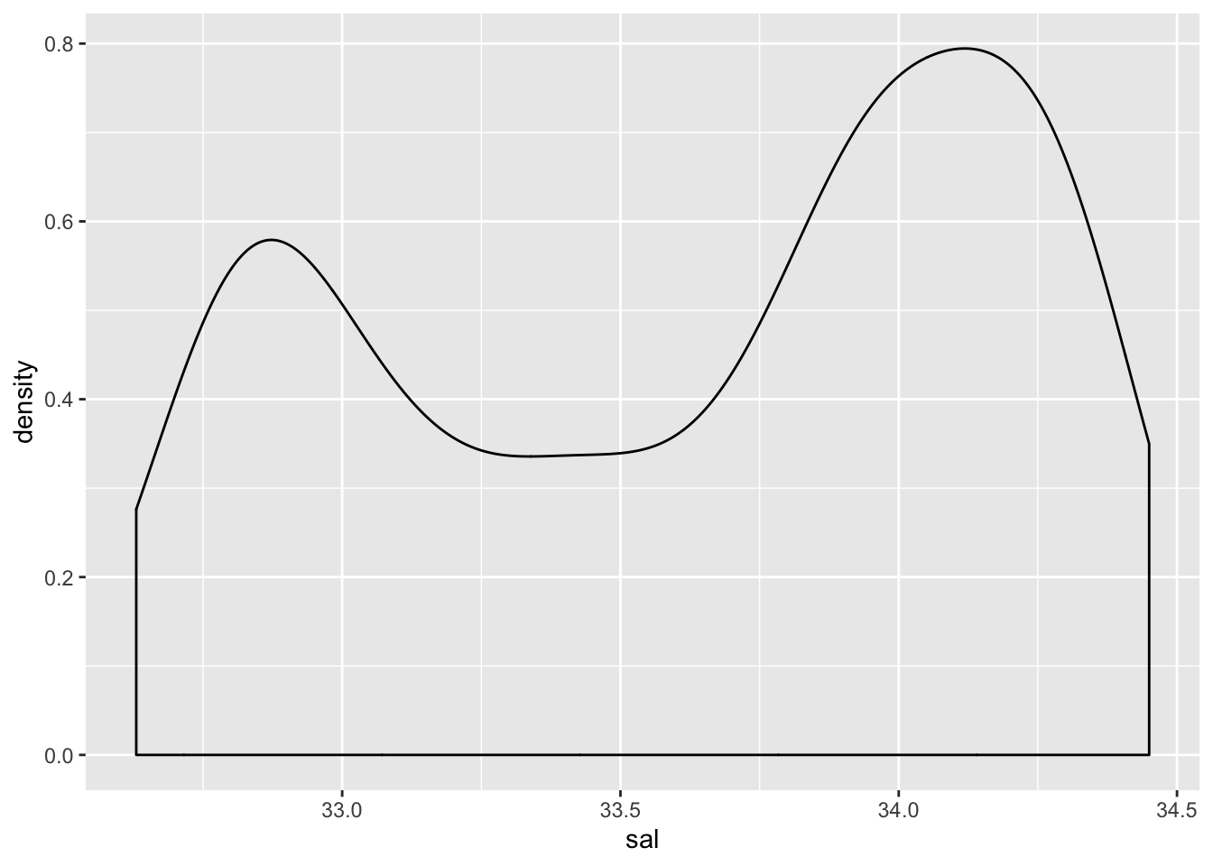
library(ggplot2)
ggplot(cofi, aes(x=temp)) + geom_density()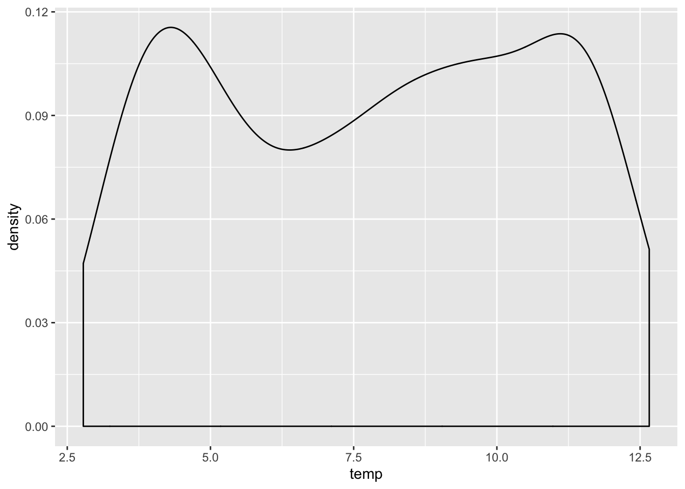
library(ggplot2)
ggplot(cofi, aes(x=depth)) + geom_density()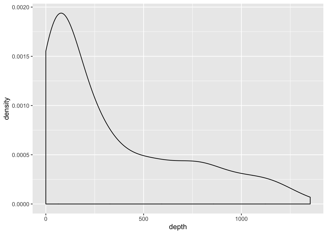
Question 3 (1pt) A scatter plot of salinity and log10(depth+1), use “salinity” as X-axis.
ggplot(cofi, aes(x=sal, y=log10(depth+1))) + geom_point() + theme_classic()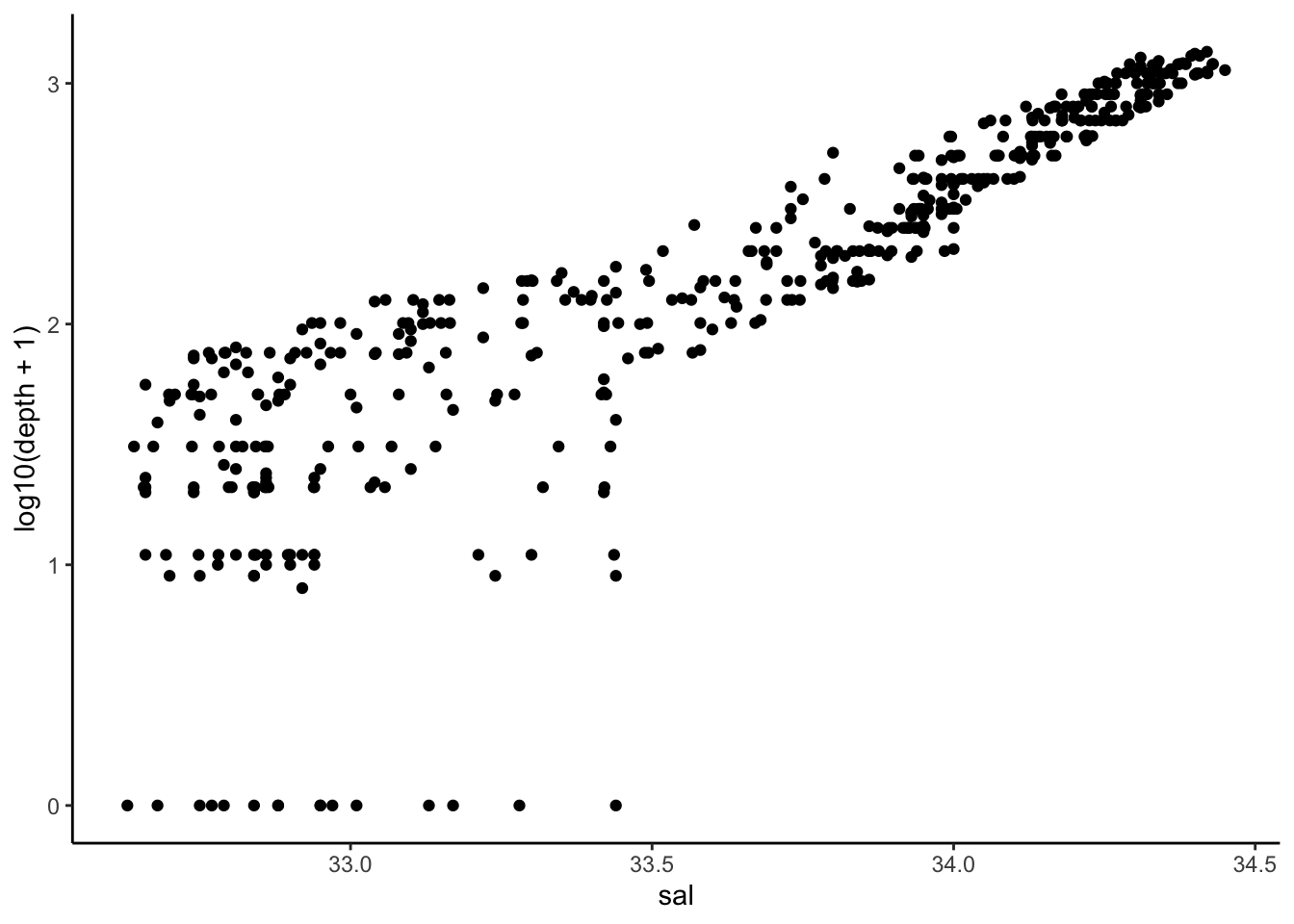
Question 4 (1pt) A correlation matrix of salinity and log10(depth+1).
cofi$log10depth <- log10(cofi$depth+1)
cor(cofi[,c(1,4)])
sal log10depth
sal 1.0000000 0.8630779
log10depth 0.8630779 1.0000000Question 5 (1pt) Use the lm() function in R, fit a simple linear regression using “salinity” as response and log10(depth+1) as predictor. Report the value of b0 and b1 in fitted simple linear regression equation.
cofi.fit <- lm(sal~log10depth, data=cofi)
summary(cofi.fit)
Call:
lm(formula = sal ~ log10depth, data = cofi)

Residuals:
     Min       1Q   Median       3Q      Max
-0.67472 -0.16683  0.07827  0.14663  1.31027

Coefficients:
            Estimate Std. Error t value Pr(>|t|)
(Intercept) 32.12973    0.04158  772.66   <2e-16 ***
log10depth   0.68744    0.01816   37.87   <2e-16 ***
---
Signif. codes:  0 '***' 0.001 '**' 0.01 '*' 0.05 '.' 0.1 ' ' 1

Residual standard error: 0.2835 on 491 degrees of freedom
Multiple R-squared:  0.7449,    Adjusted R-squared:  0.7444
F-statistic:  1434 on 1 and 491 DF,  p-value: < 2.2e-16
Question 6 (1pt) Verify the sum of the residuals equals to 0.
sum(cofi.fit$residuals)[1] 7.691764e-15Question 7 (1pt) Make a density plot for the residuals.
ggplot(cofi.fit, aes(x=cofi.fit$residuals)) + geom_density() 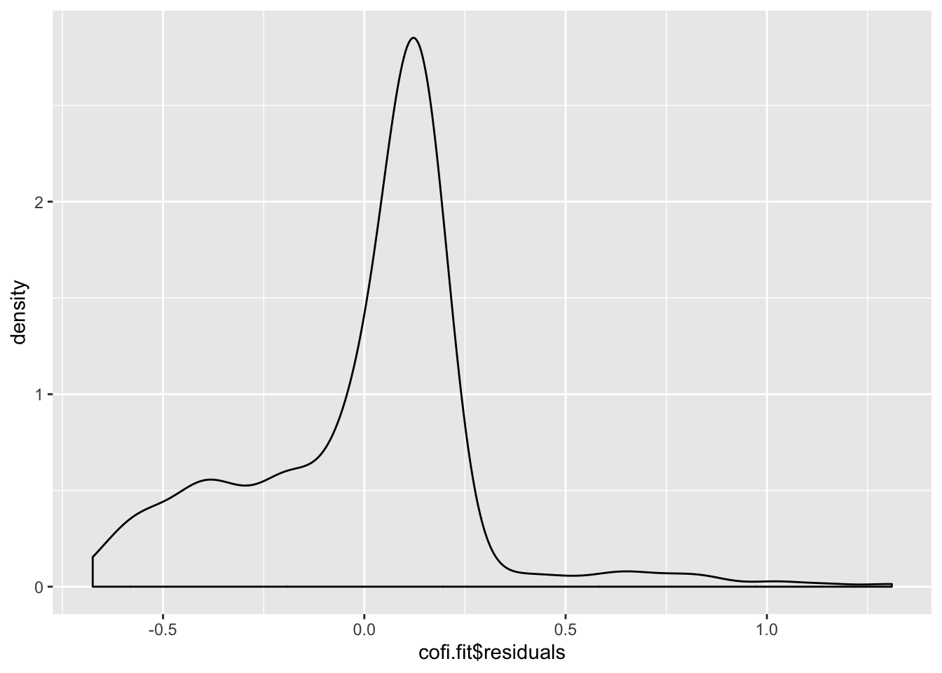
Question 8 (3pt) Instead of using lm(), use R code to calculate b0 and b1 based on the formula we discussed in class. Verify the values match the results using the lm() function.
Sxx <- sum((cofi$log10depth-mean(cofi$log10depth))^2)
Sxx
[1] 243.8907Sxy <- sum((cofi$log10depth-mean(cofi$log10depth))*(cofi$sal-mean(cofi$sal)))
Sxy[1] 167.6612b1 <- Sxy/Sxx
b1[1] 0.6874438b0 <- mean(cofi$sal)-b1*mean(cofi$log10depth)
b0[1] 32.12973
sessionInfo()R version 3.6.1 (2019-07-05)
Platform: x86_64-apple-darwin15.6.0 (64-bit)
Running under: macOS Mojave 10.14.6
Matrix products: default
BLAS: /Library/Frameworks/R.framework/Versions/3.6/Resources/lib/libRblas.0.dylib
LAPACK: /Library/Frameworks/R.framework/Versions/3.6/Resources/lib/libRlapack.dylib
locale:
[1] en_US.UTF-8/en_US.UTF-8/en_US.UTF-8/C/en_US.UTF-8/en_US.UTF-8
attached base packages:
[1] stats graphics grDevices utils datasets methods base
other attached packages:
[1] ggplot2_3.2.1
loaded via a namespace (and not attached):
[1] Rcpp_1.0.2 knitr_1.24 whisker_0.3-2 magrittr_1.5
[5] workflowr_1.4.0 tidyselect_0.2.5 munsell_0.5.0 colorspace_1.4-1
[9] R6_2.4.0 rlang_0.4.0 dplyr_0.8.3 stringr_1.4.0
[13] tools_3.6.1 grid_3.6.1 gtable_0.3.0 xfun_0.9
[17] withr_2.1.2 git2r_0.26.1 htmltools_0.3.6 assertthat_0.2.1
[21] yaml_2.2.0 lazyeval_0.2.2 rprojroot_1.3-2 digest_0.6.20
[25] tibble_2.1.3 crayon_1.3.4 purrr_0.3.2 fs_1.3.1
[29] glue_1.3.1 evaluate_0.14 rmarkdown_1.15 labeling_0.3
[33] stringi_1.4.3 pillar_1.4.2 compiler_3.6.1 scales_1.0.0
[37] backports_1.1.4 pkgconfig_2.0.2