SLR - CalCOFI data
Donghyung Lee
2019-10-01
- CalCOFI data
- Load package
- Load data
- pairwise scatter plot
- scatter plots
- SLR model, temp as a function of sal
- Add the fitted line to the scatter plot
- Summary of lm() output
- Questions
- Calculate these manually.
- Confidence Interval of beta0 and beta1
- Manually calculate CI for beta1
- Manually calculate CI for beta0
- Solutions: Calculate these manually.
Last updated: 2019-10-01
Checks: 7 0
Knit directory: STA_463_563_Fall2019/
This reproducible R Markdown analysis was created with workflowr (version 1.4.0). The Checks tab describes the reproducibility checks that were applied when the results were created. The Past versions tab lists the development history.
Great! Since the R Markdown file has been committed to the Git repository, you know the exact version of the code that produced these results.
Great job! The global environment was empty. Objects defined in the global environment can affect the analysis in your R Markdown file in unknown ways. For reproduciblity it’s best to always run the code in an empty environment.
The command set.seed(20190905) was run prior to running the code in the R Markdown file. Setting a seed ensures that any results that rely on randomness, e.g. subsampling or permutations, are reproducible.
Great job! Recording the operating system, R version, and package versions is critical for reproducibility.
Nice! There were no cached chunks for this analysis, so you can be confident that you successfully produced the results during this run.
Great job! Using relative paths to the files within your workflowr project makes it easier to run your code on other machines.
Great! You are using Git for version control. Tracking code development and connecting the code version to the results is critical for reproducibility. The version displayed above was the version of the Git repository at the time these results were generated.
Note that you need to be careful to ensure that all relevant files for the analysis have been committed to Git prior to generating the results (you can use wflow_publish or wflow_git_commit). workflowr only checks the R Markdown file, but you know if there are other scripts or data files that it depends on. Below is the status of the Git repository when the results were generated:
Ignored files:
    Ignored:    .DS_Store
    Ignored:    .Rhistory
    Ignored:    .Rproj.user/

Untracked files:
    Untracked:  analysis/lab_hw2_sol.Rmd
    Untracked:  docs/figure/lab_hw2.Rmd/
Note that any generated files, e.g. HTML, png, CSS, etc., are not included in this status report because it is ok for generated content to have uncommitted changes.
These are the previous versions of the R Markdown and HTML files. If you’ve configured a remote Git repository (see ?wflow_git_remote), click on the hyperlinks in the table below to view them.
| File | Version | Author | Date | Message |
|---|---|---|---|---|
| Rmd | 14513f7 | dleelab | 2019-09-27 | a |
| Rmd | 6f221cc | dleelab | 2019-09-27 | c |
| html | e8fc3fd | dleelab | 2019-09-27 | created |
| Rmd | 49e65ce | dleelab | 2019-09-27 | corrected |
| Rmd | e838d5a | dleelab | 2019-09-27 | q added |
| Rmd | 178c6e1 | dleelab | 2019-09-27 | added |
CalCOFI data
“The CalCOFI data set represents the longest (1949-present) and most complete (more than 50,000 sampling stations) time series of oceanographic and larval fish data in the world. It includes abundance data on the larvae of over 250 species of fish; larval length frequency data and egg abundance data on key commercial species; and oceanographic and plankton data. The physical, chemical, and biological data collected at regular time and space intervals quickly became valuable for documenting climatic cycles in the California Current and a range of biological responses to them. CalCOFI research drew world attention to the biological response to the dramatic Pacific-warming event in 1957-58 and introduced the term “El Niño” into the scientific literature."
Here, we use only 500 observations to speed up calculation.
You can download orignial data from: https://www.kaggle.com/sohier/calcofi
Load package
library(ggplot2)Load data
temp: temperature (Celsius)
sal: salinity (amount of salt dissolved in a body of water)
depth: depth (meter)
cofi <- read.table("https://raw.githubusercontent.com/dleelab/STA463_563_Fall2019/master/data/calcofi_500.csv", header=TRUE, sep = ",")
head(cofi)
sal temp depth
1 33.440 10.50 0
2 33.440 10.46 8
3 33.437 10.46 10
4 33.420 10.45 19
5 33.421 10.45 20
6 33.431 10.45 30dim(cofi)[1] 493 3summary(cofi) sal temp depth
Min. :32.63 Min. : 2.780 Min. : 0
1st Qu.:33.07 1st Qu.: 5.020 1st Qu.: 62
Median :33.80 Median : 8.120 Median : 200
Mean :33.63 Mean : 7.821 Mean : 345
3rd Qu.:34.13 3rd Qu.:10.450 3rd Qu.: 600
Max. :34.45 Max. :12.660 Max. :1352 pairwise scatter plot
pairs(cofi)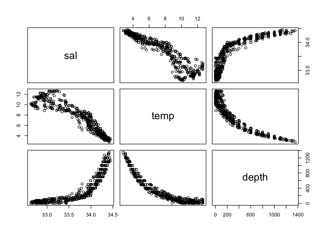
| Version | Author | Date |
|---|---|---|
| e8fc3fd | dleelab | 2019-09-27 |
cor(cofi) sal temp depth
sal 1.0000000 -0.9229002 0.8363158
temp -0.9229002 1.0000000 -0.9105742
depth 0.8363158 -0.9105742 1.0000000scatter plots
# temperature as a function of salinity
ggplot(cofi, aes(x=sal, y=temp, col=depth)) +
  geom_point() +
  labs(x="Salinity", y="Temperature(C)", col = "Depth(m)")+
  theme_classic()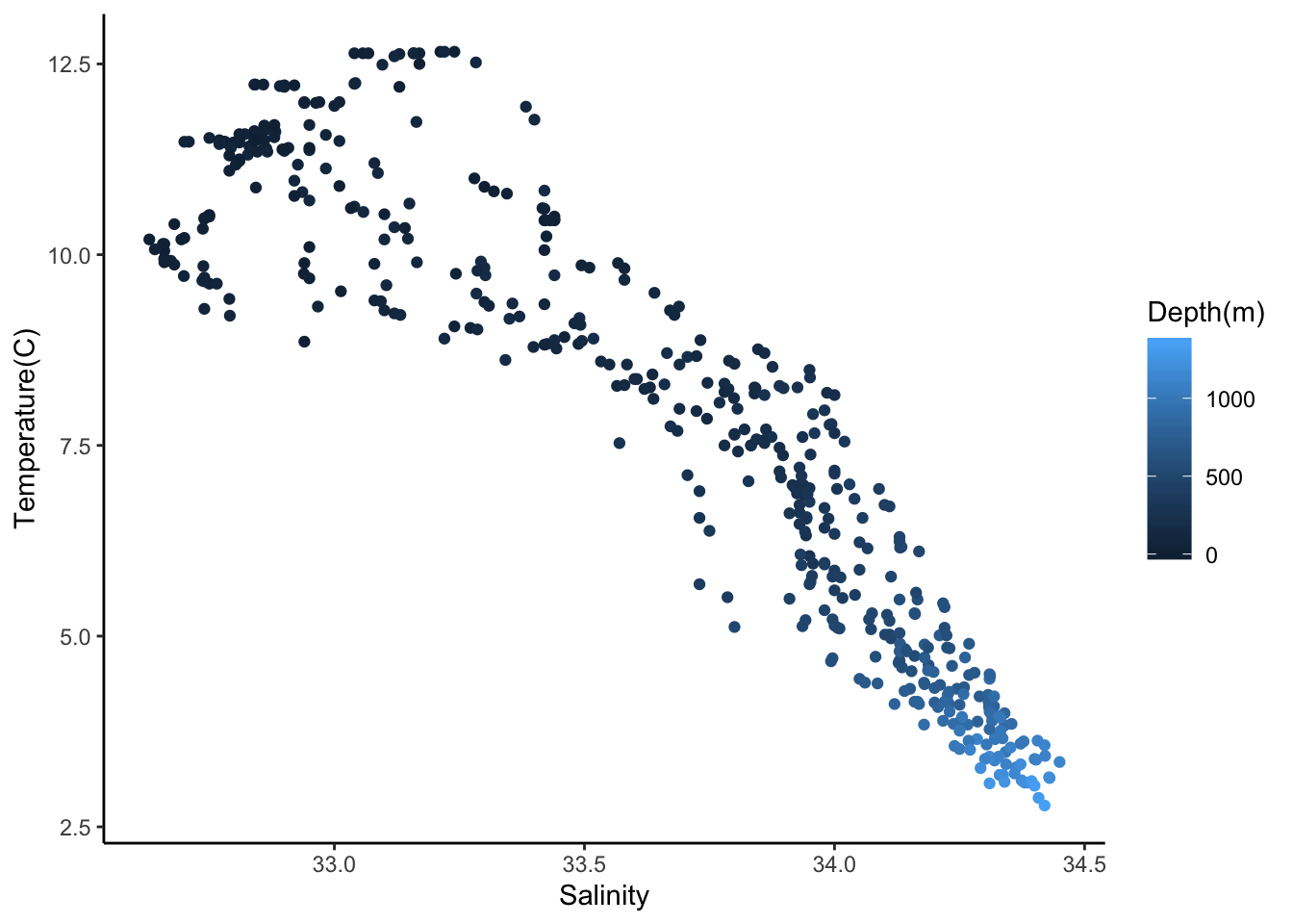
| Version | Author | Date |
|---|---|---|
| e8fc3fd | dleelab | 2019-09-27 |
#salinity as a function of depth
ggplot(cofi, aes(x=depth, y=sal, col=temp)) +
  geom_point() +
  labs(x="Depth(m)", y="Salinity", col = "Temperature(C)")+
  theme_classic()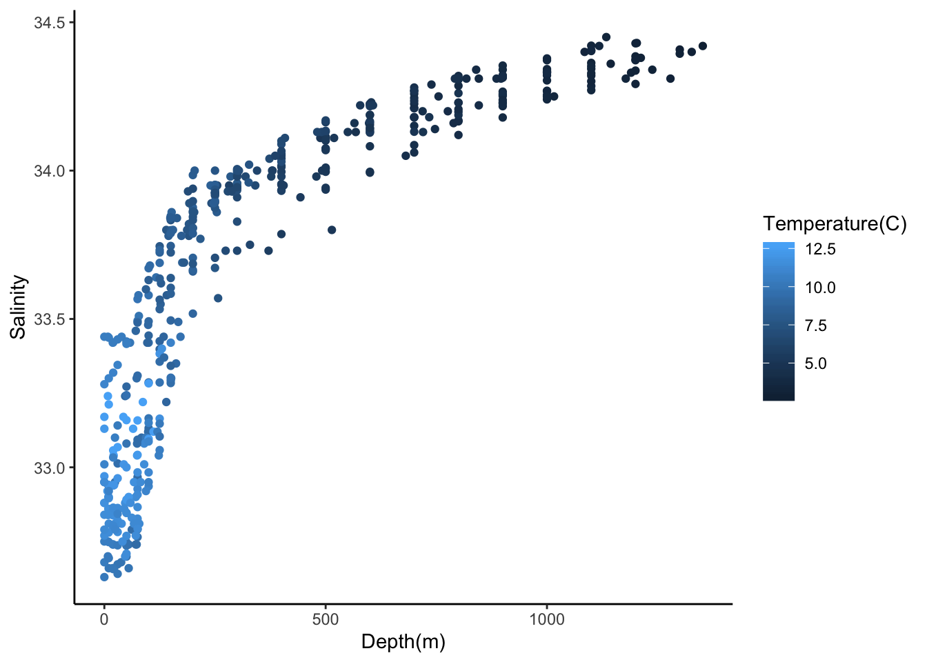
| Version | Author | Date |
|---|---|---|
| e8fc3fd | dleelab | 2019-09-27 |
#salinity as a function of log10(depth)
ggplot(cofi, aes(x=log10(depth), y=sal, col=temp)) +
  geom_point() +
  labs(x="log10(Depth(m))", y="Salinity", col = "Temperature(C)")+
  theme_classic()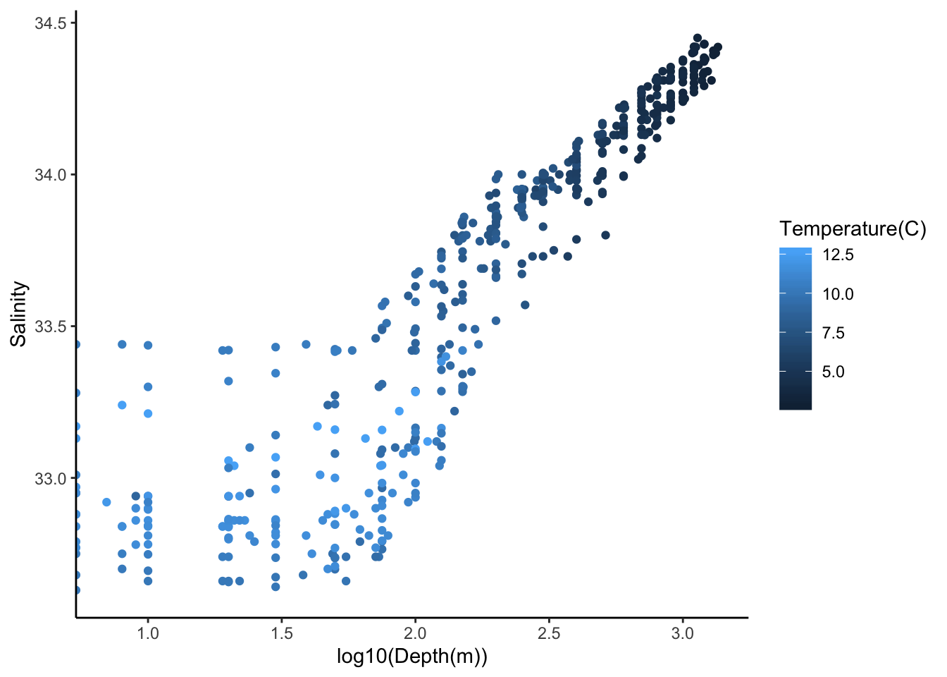
| Version | Author | Date |
|---|---|---|
| e8fc3fd | dleelab | 2019-09-27 |
SLR model, temp as a function of sal
cofi.fit <- lm(temp~sal,data=cofi)
cofi.fit
Call:
lm(formula = temp ~ sal, data = cofi)

Coefficients:
(Intercept)          sal
    169.118       -4.796
Add the fitted line to the scatter plot
ggplot(cofi, aes(x=sal, y=temp, col=depth)) +
  geom_point() +
  geom_smooth(method='lm') +
  labs(x="Salinity", y="Temperature(C)", col = "Depth(m)")+
  theme_classic()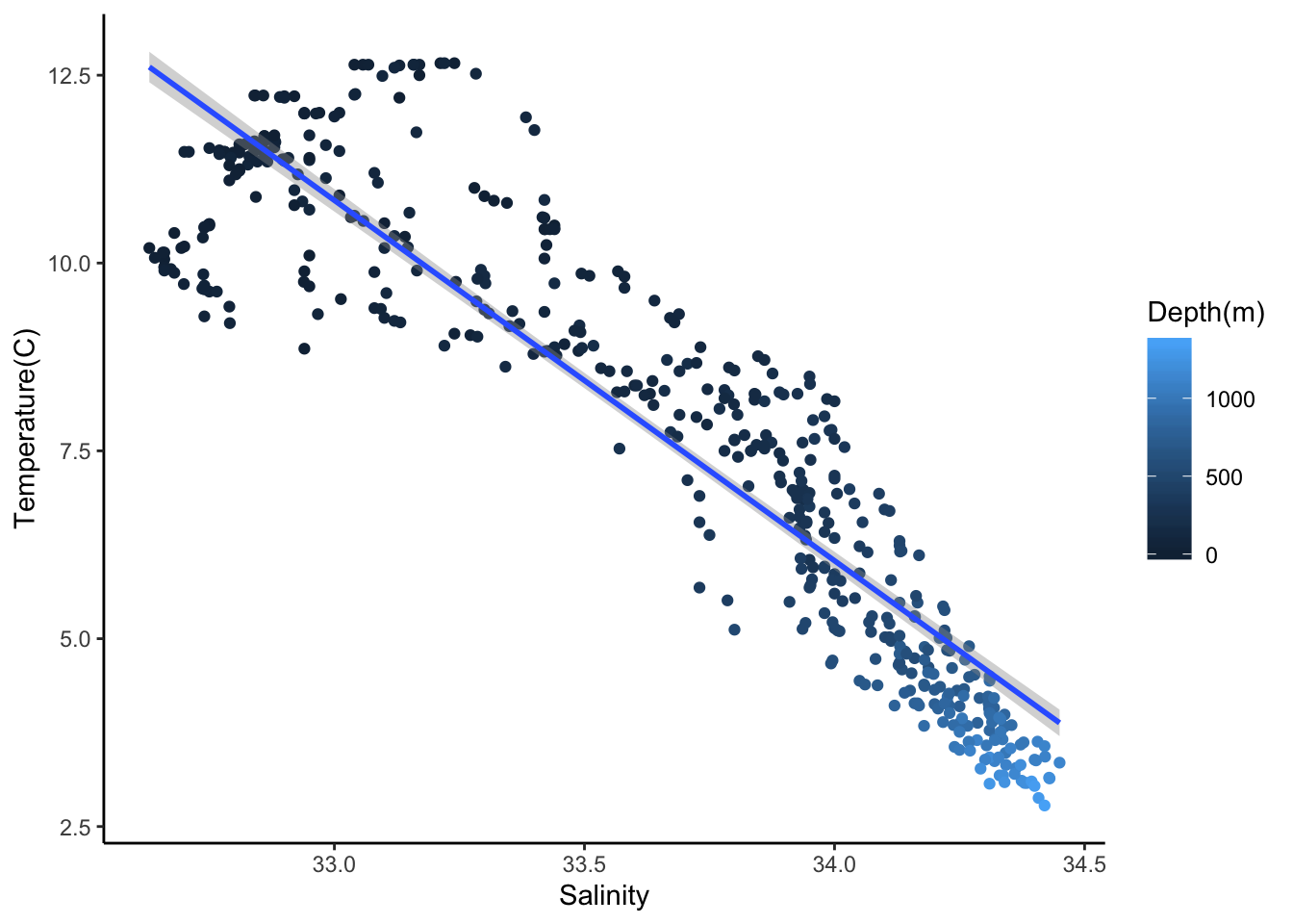
| Version | Author | Date |
|---|---|---|
| e8fc3fd | dleelab | 2019-09-27 |
Summary of lm() output
summary(cofi.fit)
Call:
lm(formula = temp ~ sal, data = cofi)

Residuals:
     Min       1Q   Median       3Q      Max
-2.79153 -0.75022 -0.06611  0.66100  3.04295

Coefficients:
             Estimate Std. Error t value Pr(>|t|)
(Intercept) 169.11780    3.03735   55.68   <2e-16 ***
sal          -4.79646    0.09031  -53.11   <2e-16 ***
---
Signif. codes:  0 '***' 0.001 '**' 0.01 '*' 0.05 '.' 0.1 ' ' 1

Residual standard error: 1.123 on 491 degrees of freedom
Multiple R-squared:  0.8517,    Adjusted R-squared:  0.8514
F-statistic:  2821 on 1 and 491 DF,  p-value: < 2.2e-16
Questions
Q1. What is sample size?
Q2. What is b0 value?
Q3. What is b1 value?
Q4. What is fitted regression line?
Q5. Test statistic value for a hypothesis test on Beta0 ?
Q6. Test statistic value for a hypothesis test on Beta1?
Q7. What is MSE?
Calculate these manually.
# Residual
# Sum of residuals
# Residual Sum of Squares
# SSE
# DF
# MSE
# Residual Standard Error: sqrt(MSE)
# cor(sal, temp)
# Sxx
# Syy
# Compute cor(sal, temp) using b1, Sxx and Syy
Confidence Interval of beta0 and beta1
confint(cofi.fit) 2.5 % 97.5 %
(Intercept) 163.149993 175.085599
sal -4.973905 -4.619025Manually calculate CI for beta1
# b1 +- T(1-alpha/2,n-2)*sqrt(MSE/Sxx)
MSE <- sum(cofi.fit$residuals^2)/cofi.fit$df.residual
Sxx <- sum((cofi$sal-mean(cofi$sal))^2)
tval <- qt(.975, df=cofi.fit$df.residual)

cofi.fit$coefficients[2]-tval*sqrt(MSE/Sxx) #lower bound
sal
-4.973905 cofi.fit$coefficients[2]+tval*sqrt(MSE/Sxx) #upper bound sal
-4.619025 Manually calculate CI for beta0
# b1 +- T(1-alpha/2,n-2)*sqrt(MSE*(1/n+mean(x)^2/Sxx))
MSE <- sum(cofi.fit$residuals^2)/cofi.fit$df.residual
Sxx <- sum((cofi$sal-mean(cofi$sal))^2)
n <- nrow(cofi)
tval <- qt(.975, df=cofi.fit$df.residual)

cofi.fit$coefficients[1]-tval*sqrt(MSE*(1/n+mean(cofi$sal)^2/Sxx)) #lower bound
(Intercept)
163.15 cofi.fit$coefficients[1]+tval*sqrt(MSE*(1/n+mean(cofi$sal)^2/Sxx)) #upper bound(Intercept)
175.0856 Solutions: Calculate these manually.
# Residual
hist(cofi.fit$residuals)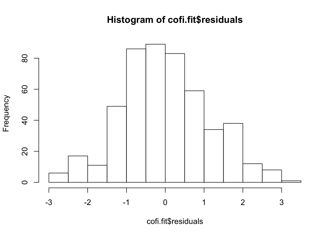
| Version | Author | Date |
|---|---|---|
| e8fc3fd | dleelab | 2019-09-27 |
plot(density(cofi.fit$residuals), xlab="Residuals")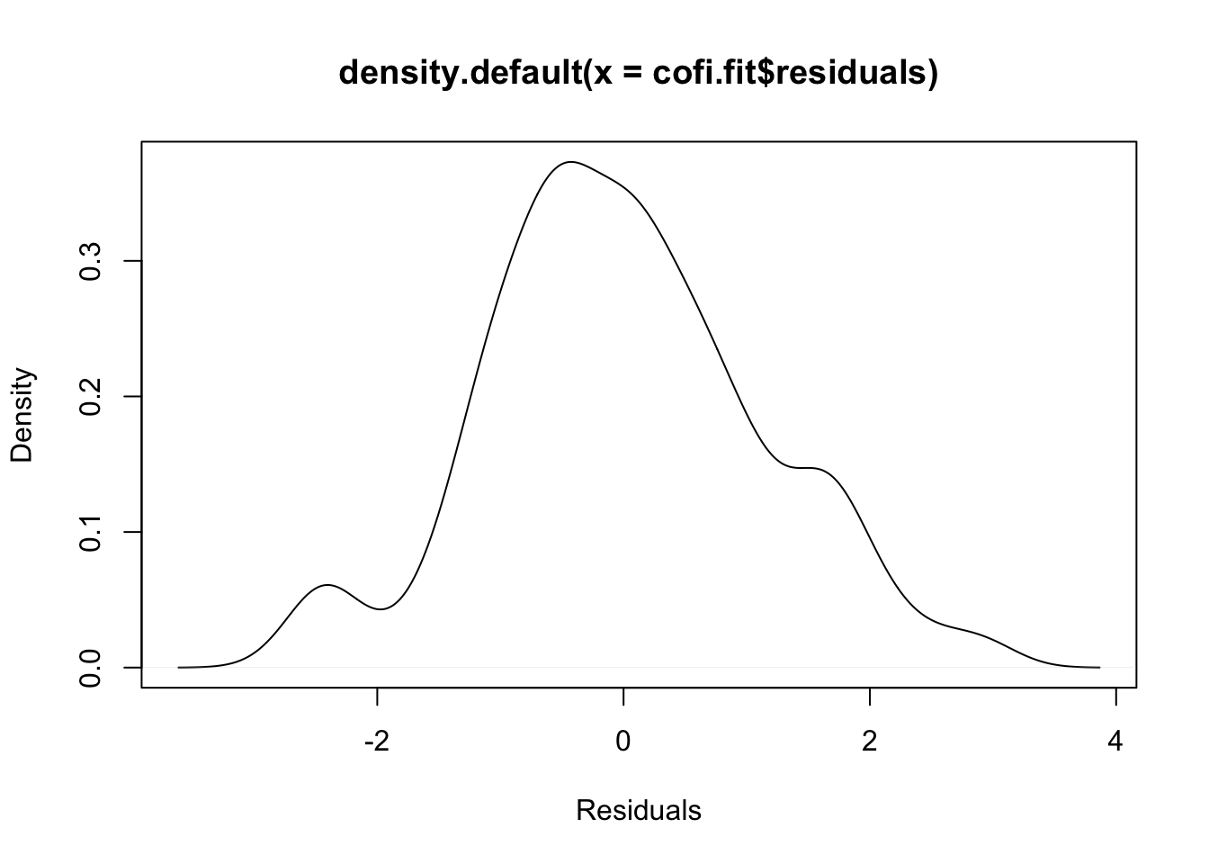
# Sum of residuals
sum(cofi.fit$residuals)
[1] 3.298056e-14# Residual Sum of Squares
RSS <- sum(cofi.fit$residuals^2)
# SSE
SSE <- sum(cofi.fit$residuals^2)
# DF
DF <- cofi.fit$df.residual
# MSE
MSE <- SSE/DF
# Residual Standard Error: sqrt(MSE)
RSE <- sqrt(MSE)
# cor(sal, temp)
cor(cofi$sal, cofi$temp)[1] -0.9229002# Sxx
Sxx <- sum((cofi$sal-mean(cofi$sal))^2)
# Syy
Syy <- sum((cofi$temp-mean(cofi$temp))^2)
# Compute cor(sal, temp) using b1, Sxx and Syy
r <- cofi.fit$coefficients[2]*sqrt(Sxx/Syy)
r sal
-0.9229002 cor(cofi$sal, cofi$temp)[1] -0.9229002
sessionInfo()R version 3.6.1 (2019-07-05)
Platform: x86_64-apple-darwin15.6.0 (64-bit)
Running under: macOS Mojave 10.14.6
Matrix products: default
BLAS: /Library/Frameworks/R.framework/Versions/3.6/Resources/lib/libRblas.0.dylib
LAPACK: /Library/Frameworks/R.framework/Versions/3.6/Resources/lib/libRlapack.dylib
locale:
[1] en_US.UTF-8/en_US.UTF-8/en_US.UTF-8/C/en_US.UTF-8/en_US.UTF-8
attached base packages:
[1] stats graphics grDevices utils datasets methods base
other attached packages:
[1] ggplot2_3.2.1
loaded via a namespace (and not attached):
[1] Rcpp_1.0.2 knitr_1.24 whisker_0.3-2 magrittr_1.5
[5] workflowr_1.4.0 tidyselect_0.2.5 munsell_0.5.0 colorspace_1.4-1
[9] R6_2.4.0 rlang_0.4.0 dplyr_0.8.3 stringr_1.4.0
[13] tools_3.6.1 grid_3.6.1 gtable_0.3.0 xfun_0.9
[17] withr_2.1.2 git2r_0.26.1 htmltools_0.3.6 assertthat_0.2.1
[21] yaml_2.2.0 lazyeval_0.2.2 rprojroot_1.3-2 digest_0.6.20
[25] tibble_2.1.3 crayon_1.3.4 purrr_0.3.2 fs_1.3.1
[29] glue_1.3.1 evaluate_0.14 rmarkdown_1.15 labeling_0.3
[33] stringi_1.4.3 pillar_1.4.2 compiler_3.6.1 scales_1.0.0
[37] backports_1.1.4 pkgconfig_2.0.2