Simple Linear Regression Model
Donghyung Lee
2019-09-20
Last updated: 2019-09-20
Checks: 7 0
Knit directory: STA_463_563_Fall2019/
This reproducible R Markdown analysis was created with workflowr (version 1.4.0). The Checks tab describes the reproducibility checks that were applied when the results were created. The Past versions tab lists the development history.
Great! Since the R Markdown file has been committed to the Git repository, you know the exact version of the code that produced these results.
Great job! The global environment was empty. Objects defined in the global environment can affect the analysis in your R Markdown file in unknown ways. For reproduciblity it’s best to always run the code in an empty environment.
The command set.seed(20190905) was run prior to running the code in the R Markdown file. Setting a seed ensures that any results that rely on randomness, e.g. subsampling or permutations, are reproducible.
Great job! Recording the operating system, R version, and package versions is critical for reproducibility.
Nice! There were no cached chunks for this analysis, so you can be confident that you successfully produced the results during this run.
Great job! Using relative paths to the files within your workflowr project makes it easier to run your code on other machines.
Great! You are using Git for version control. Tracking code development and connecting the code version to the results is critical for reproducibility. The version displayed above was the version of the Git repository at the time these results were generated.
Note that you need to be careful to ensure that all relevant files for the analysis have been committed to Git prior to generating the results (you can use wflow_publish or wflow_git_commit). workflowr only checks the R Markdown file, but you know if there are other scripts or data files that it depends on. Below is the status of the Git repository when the results were generated:
Ignored files:
    Ignored:    .DS_Store
    Ignored:    .Rhistory
    Ignored:    .Rproj.user/

Untracked files:
    Untracked:  docs/figure/slr_prac.Rmd/

Unstaged changes:
    Modified:   analysis/lab2_inclass_prac.Rmd
Note that any generated files, e.g. HTML, png, CSS, etc., are not included in this status report because it is ok for generated content to have uncommitted changes.
These are the previous versions of the R Markdown and HTML files. If you’ve configured a remote Git repository (see ?wflow_git_remote), click on the hyperlinks in the table below to view them.
| File | Version | Author | Date | Message |
|---|---|---|---|---|
| Rmd | 7f66afb | dleelab | 2019-09-20 | created |
Load data
library(ggplot2)
copier <- read.table("data/CH01PR20.txt")
dim(copier)
[1] 45 2colnames(copier)=c("minutes","number")Simple Linear Regression
copier.fit <- lm(minutes~number,data=copier)
copier.fit
Call:
lm(formula = minutes ~ number, data = copier)

Coefficients:
(Intercept)       number
-0.5802 15.0352 class(copier.fit)[1] "lm"str(copier.fit)List of 12
$ coefficients : Named num [1:2] -0.58 15.04
..- attr(*, "names")= chr [1:2] "(Intercept)" "number"
$ residuals : Named num [1:45] -9.49 0.439 1.474 11.51 -2.455 ...
..- attr(*, "names")= chr [1:45] "1" "2" "3" "4" ...
$ effects : Named num [1:45] -511.61 277.42 2.56 12.5 -1.55 ...
..- attr(*, "names")= chr [1:45] "(Intercept)" "number" "" "" ...
$ rank : int 2
$ fitted.values: Named num [1:45] 29.5 59.6 44.5 29.5 14.5 ...
..- attr(*, "names")= chr [1:45] "1" "2" "3" "4" ...
$ assign : int [1:2] 0 1
$ qr :List of 5
..$ qr : num [1:45, 1:2] -6.708 0.149 0.149 0.149 0.149 ...
.. ..- attr(*, "dimnames")=List of 2
.. .. ..$ : chr [1:45] "1" "2" "3" "4" ...
.. .. ..$ : chr [1:2] "(Intercept)" "number"
.. ..- attr(*, "assign")= int [1:2] 0 1
..$ qraux: num [1:2] 1.15 1.04
..$ pivot: int [1:2] 1 2
..$ tol : num 1e-07
..$ rank : int 2
..- attr(*, "class")= chr "qr"
$ df.residual : int 43
$ xlevels : Named list()
$ call : language lm(formula = minutes ~ number, data = copier)
$ terms :Classes 'terms', 'formula' language minutes ~ number
.. ..- attr(*, "variables")= language list(minutes, number)
.. ..- attr(*, "factors")= int [1:2, 1] 0 1
.. .. ..- attr(*, "dimnames")=List of 2
.. .. .. ..$ : chr [1:2] "minutes" "number"
.. .. .. ..$ : chr "number"
.. ..- attr(*, "term.labels")= chr "number"
.. ..- attr(*, "order")= int 1
.. ..- attr(*, "intercept")= int 1
.. ..- attr(*, "response")= int 1
.. ..- attr(*, ".Environment")=<environment: R_GlobalEnv>
.. ..- attr(*, "predvars")= language list(minutes, number)
.. ..- attr(*, "dataClasses")= Named chr [1:2] "numeric" "numeric"
.. .. ..- attr(*, "names")= chr [1:2] "minutes" "number"
$ model :'data.frame': 45 obs. of 2 variables:
..$ minutes: int [1:45] 20 60 46 41 12 137 68 89 4 32 ...
..$ number : int [1:45] 2 4 3 2 1 10 5 5 1 2 ...
..- attr(*, "terms")=Classes 'terms', 'formula' language minutes ~ number
.. .. ..- attr(*, "variables")= language list(minutes, number)
.. .. ..- attr(*, "factors")= int [1:2, 1] 0 1
.. .. .. ..- attr(*, "dimnames")=List of 2
.. .. .. .. ..$ : chr [1:2] "minutes" "number"
.. .. .. .. ..$ : chr "number"
.. .. ..- attr(*, "term.labels")= chr "number"
.. .. ..- attr(*, "order")= int 1
.. .. ..- attr(*, "intercept")= int 1
.. .. ..- attr(*, "response")= int 1
.. .. ..- attr(*, ".Environment")=<environment: R_GlobalEnv>
.. .. ..- attr(*, "predvars")= language list(minutes, number)
.. .. ..- attr(*, "dataClasses")= Named chr [1:2] "numeric" "numeric"
.. .. .. ..- attr(*, "names")= chr [1:2] "minutes" "number"
- attr(*, "class")= chr "lm"summary(copier.fit)
Call:
lm(formula = minutes ~ number, data = copier)

Residuals:
     Min       1Q   Median       3Q      Max
-22.7723  -3.7371   0.3334   6.3334  15.4039

Coefficients:
            Estimate Std. Error t value Pr(>|t|)
(Intercept)  -0.5802     2.8039  -0.207    0.837
number       15.0352     0.4831  31.123   <2e-16 ***
---
Signif. codes:  0 '***' 0.001 '**' 0.01 '*' 0.05 '.' 0.1 ' ' 1

Residual standard error: 8.914 on 43 degrees of freedom
Multiple R-squared:  0.9575,    Adjusted R-squared:  0.9565
F-statistic: 968.7 on 1 and 43 DF,  p-value: < 2.2e-16
Fitted regression line (traditional R functions)
plot(minutes~number, data=copier)
abline(-0.5802,15.0352)#by definition of the line abline(intercept, slope)

#The following are alternative ways to draw the fitted regression line.
lines(copier$number,-0.5802+15.0352*copier$number)#other way

abline(copier.fit)#simple way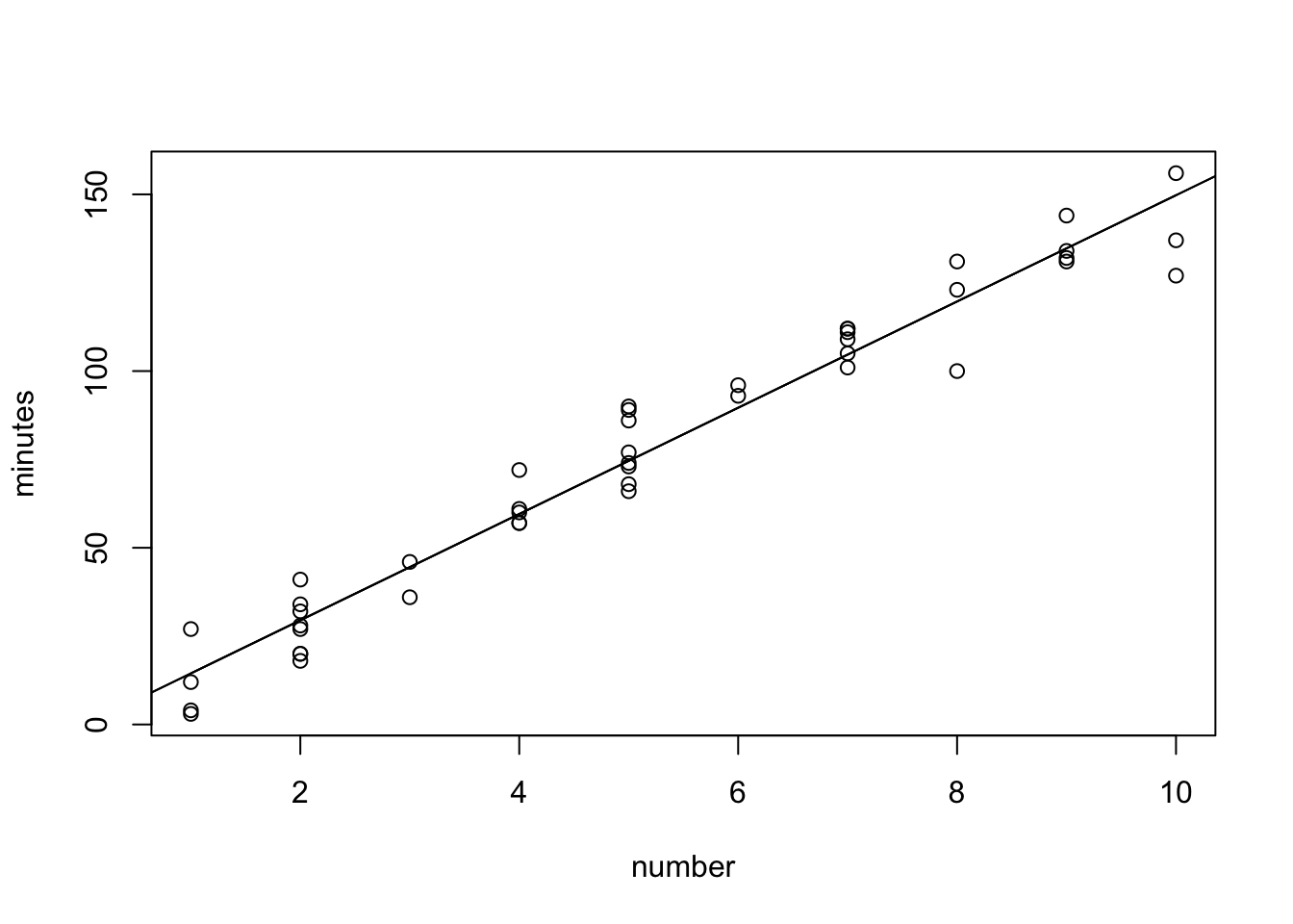
Fitted regression line (ggplot2)
fitted(copier.fit) 1 2 3 4 5 6 7
29.49034 59.56084 44.52559 29.49034 14.45509 149.77232 74.59608
8 9 10 11 12 13 14
74.59608 14.45509 29.49034 134.73708 149.77232 89.63133 44.52559
15 16 17 18 19 20 21
59.56084 119.70183 104.66658 119.70183 149.77232 59.56084 74.59608
22 23 24 25 26 27 28
104.66658 104.66658 74.59608 134.73708 104.66658 29.49034 74.59608
29 30 31 32 33 34 35
104.66658 89.63133 119.70183 74.59608 29.49034 29.49034 14.45509
36 37 38 39 40 41 42
59.56084 74.59608 134.73708 104.66658 14.45509 134.73708 29.49034
43 44 45
29.49034 59.56084 74.59608 copier$fitted=fitted(copier.fit)
p <- ggplot(copier,aes(x=number, y=minutes)) +
geom_point()
p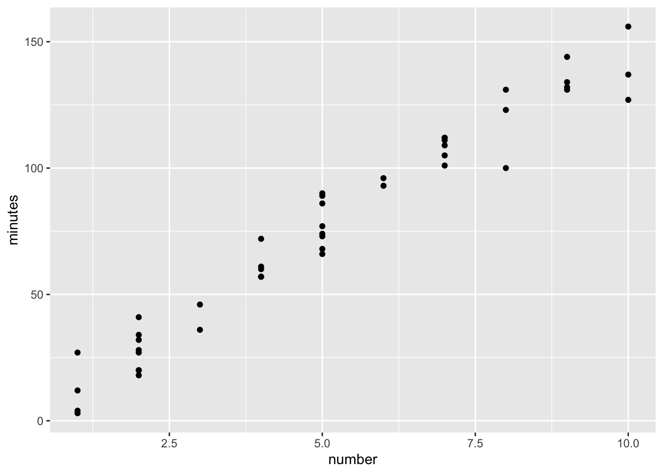
p <- p + geom_line(aes(x=number,y=fitted))
p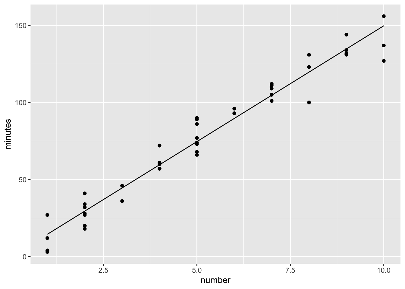
Results of lm()
Verify the lm() gives us the correct calculation result
- Residual standard error=sqrt(MSE)=sqrt(SSE/n-2), n-2 is the degree of freedom. We can verify this later.
- It gives a five number summary of the residuals, mean of residuals is? It’s 0. We proved this during class.
- Since residuals are estimates of errors, under normal error SLR, we expect the residuals are also normally distributed. Are the residuals normally distribued?
Question 1. How to get the residuals?
Question 2. How to get the estimated values? Are there other measures already calculated?
Attributes of fitted model
attributes(copier.fit)#There're many measures calculated by lm function. $names
[1] "coefficients" "residuals" "effects" "rank"
[5] "fitted.values" "assign" "qr" "df.residual"
[9] "xlevels" "call" "terms" "model"
$class
[1] "lm"Residuals
#For example, you can look at the residuals.
#Verify the residual standard error, degree of freedom is correct.
summary(copier.fit)
Call:
lm(formula = minutes ~ number, data = copier)

Residuals:
     Min       1Q   Median       3Q      Max
-22.7723  -3.7371   0.3334   6.3334  15.4039

Coefficients:
            Estimate Std. Error t value Pr(>|t|)
(Intercept)  -0.5802     2.8039  -0.207    0.837
number       15.0352     0.4831  31.123   <2e-16 ***
---
Signif. codes:  0 '***' 0.001 '**' 0.01 '*' 0.05 '.' 0.1 ' ' 1

Residual standard error: 8.914 on 43 degrees of freedom
Multiple R-squared:  0.9575,    Adjusted R-squared:  0.9565
F-statistic: 968.7 on 1 and 43 DF,  p-value: < 2.2e-16
res=copier.fit$residuals
SSE=sum(res^2)
df=nrow(copier)-2
MSE=SSE/df
sqrt(MSE) # Residual standard error[1] 8.913508c(SSE,df,MSE,sqrt(MSE))[1] 3416.377023 43.000000 79.450628 8.913508Distribution of residauls
#Have an idea whether the residuals have a normal distribution.
plot(density(copier.fit$residuals),xlab="Residuals")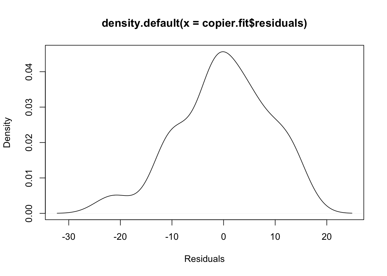
#which observaiton has the smallest residual (in absolute value)
absres=abs(res)

pos=which(absres==min(absres))
pos=which.min(absres) #an alternative way

copier.fit$fitted.values[pos]#the fitted value corresponding to this point
17
104.6666 copier[pos,1]#the observed response of this observation[1] 105# what is residual?Practice
plot(iris$Sepal.Length, iris$Petal.Length)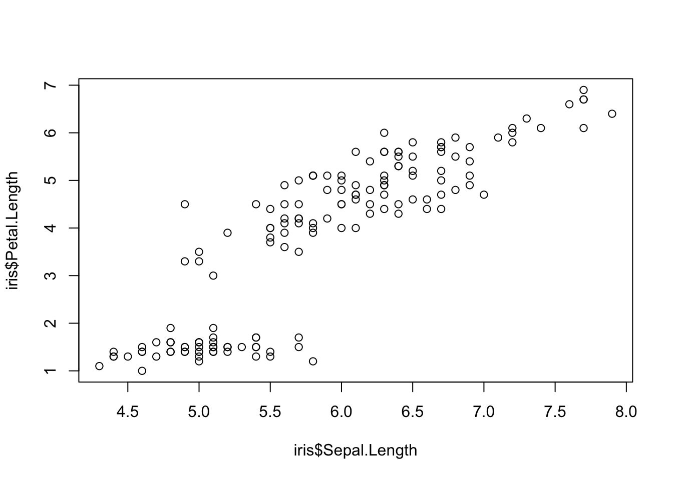
iris.fit <- lm(Sepal.Length~Petal.Length,data=iris)
summary(iris.fit)
Call:
lm(formula = Sepal.Length ~ Petal.Length, data = iris)

Residuals:
     Min       1Q   Median       3Q      Max
-1.24675 -0.29657 -0.01515  0.27676  1.00269

Coefficients:
             Estimate Std. Error t value Pr(>|t|)
(Intercept)   4.30660    0.07839   54.94   <2e-16 ***
Petal.Length  0.40892    0.01889   21.65   <2e-16 ***
---
Signif. codes:  0 '***' 0.001 '**' 0.01 '*' 0.05 '.' 0.1 ' ' 1

Residual standard error: 0.4071 on 148 degrees of freedom
Multiple R-squared:   0.76, Adjusted R-squared:  0.7583
F-statistic: 468.6 on 1 and 148 DF,  p-value: < 2.2e-16
## Add fitted line in the scatter plot.
## SSE, df, MSE, RSE ?
## distribution of residuals ?Beta0=0
We can force Beta0 = 0. We do this in R by telling the lm() function to not include an intercept. We can do this with the 0 + option or the -1 option. See the examples below.
lm(minutes ~ number, data=copier)
Call:
lm(formula = minutes ~ number, data = copier)

Coefficients:
(Intercept)       number
    -0.5802      15.0352
lm(minutes ~ 0 + number, data=copier)
Call:
lm(formula = minutes ~ 0 + number, data = copier)

Coefficients:
number
 14.95
lm(minutes ~ -1 + number, data=copier)
Call:
lm(formula = minutes ~ -1 + number, data = copier)

Coefficients:
number
 14.95
Beta1=0
Likewise, we could use the lm() function to fit a model with no slope, but specifying the predictor variables to be constants
# when Beta1 = 0.
lm(Sepal.Length ~ 1, data=iris)
Call:
lm(formula = Sepal.Length ~ 1, data = iris)

Coefficients:
(Intercept)
      5.843
sessionInfo()R version 3.6.1 (2019-07-05)
Platform: x86_64-apple-darwin15.6.0 (64-bit)
Running under: macOS Mojave 10.14.6
Matrix products: default
BLAS: /Library/Frameworks/R.framework/Versions/3.6/Resources/lib/libRblas.0.dylib
LAPACK: /Library/Frameworks/R.framework/Versions/3.6/Resources/lib/libRlapack.dylib
locale:
[1] en_US.UTF-8/en_US.UTF-8/en_US.UTF-8/C/en_US.UTF-8/en_US.UTF-8
attached base packages:
[1] stats graphics grDevices utils datasets methods base
other attached packages:
[1] ggplot2_3.2.1
loaded via a namespace (and not attached):
[1] Rcpp_1.0.2 knitr_1.24 whisker_0.3-2 magrittr_1.5
[5] workflowr_1.4.0 tidyselect_0.2.5 munsell_0.5.0 colorspace_1.4-1
[9] R6_2.4.0 rlang_0.4.0 dplyr_0.8.3 stringr_1.4.0
[13] tools_3.6.1 grid_3.6.1 gtable_0.3.0 xfun_0.9
[17] withr_2.1.2 git2r_0.26.1 htmltools_0.3.6 assertthat_0.2.1
[21] yaml_2.2.0 lazyeval_0.2.2 rprojroot_1.3-2 digest_0.6.20
[25] tibble_2.1.3 crayon_1.3.4 purrr_0.3.2 fs_1.3.1
[29] glue_1.3.1 evaluate_0.14 rmarkdown_1.15 labeling_0.3
[33] stringi_1.4.3 pillar_1.4.2 compiler_3.6.1 scales_1.0.0
[37] backports_1.1.4 pkgconfig_2.0.2