Transformation

workflowr

• Summary
• Checks
• Past versions

Last updated: 2019-11-15

Checks: 7 0

Knit directory: STA_463_563_Fall2019/

This reproducible R Markdown analysis was created with workflowr (version 1.4.0). The Checks tab describes the reproducibility checks that were applied when the results were created. The Past versions tab lists the development history.

---

R Markdown file: up-to-date

Great! Since the R Markdown file has been committed to the Git repository, you know the exact version of the code that produced these results.

Environment: empty

Great job! The global environment was empty. Objects defined in the global environment can affect the analysis in your R Markdown file in unknown ways. For reproduciblity it’s best to always run the code in an empty environment.

Seed: set.seed(20190905)

The command set.seed(20190905) was run prior to running the code in the R Markdown file. Setting a seed ensures that any results that rely on randomness, e.g. subsampling or permutations, are reproducible.

Session information: recorded

Great job! Recording the operating system, R version, and package versions is critical for reproducibility.

Cache: none

Nice! There were no cached chunks for this analysis, so you can be confident that you successfully produced the results during this run.

File paths: relative

Great job! Using relative paths to the files within your workflowr project makes it easier to run your code on other machines.

Repository version: ed05c7b

Great! You are using Git for version control. Tracking code development and connecting the code version to the results is critical for reproducibility. The version displayed above was the version of the Git repository at the time these results were generated.

Note that you need to be careful to ensure that all relevant files for the analysis have been committed to Git prior to generating the results (you can use wflow_publish or wflow_git_commit). workflowr only checks the R Markdown file, but you know if there are other scripts or data files that it depends on. Below is the status of the Git repository when the results were generated:

Ignored files:
    Ignored:    .DS_Store
    Ignored:    .Rhistory
    Ignored:    .Rproj.user/
    Ignored:    analysis/.DS_Store

Untracked files:
    Untracked:  docs/figure/transform.Rmd/

Note that any generated files, e.g. HTML, png, CSS, etc., are not included in this status report because it is ok for generated content to have uncommitted changes.

---

These are the previous versions of the R Markdown and HTML files. If you’ve configured a remote Git repository (see ?wflow_git_remote), click on the hyperlinks in the table below to view them.

File	Version	Author	Date	Message
Rmd	ed05c7b	dleelab	2019-11-15	created

---

Non-normal errors and Non-constant error variance

Transformations of the response variable Y can improve the fit and correct violations of model assumptions such as normality and constant error variance.

• Normality:
  • Thanks to the Central Limit Theorem, we can actually get away with some mild violation of the normality assumption when ths sample size is large.
  • If your sample is small, the normality assumption is pretty important.
• Constant Variance:
  • For test and CI or PI results to be correct, we must assume that the variance of the errors is constant.
  • It is usually a more crucial assumption than normality in validating model inferences.

Box-Cox Method: Transformations of the response variable Y

• The Box-Cox transformation method is a popular way to determine a normalizing data transformation for Y.

• It is designed for strictly positive responses \((Y > 0)\) and determines the transformation to find the best fit to the data.

• In the Box-Cox method, instead of fitting the original Y as the response, we determine a transformed version \(t_{\lambda}(Y)\), where

\[ \begin{aligned} t_{\lambda}(Y)=\left \{\begin{array}{ll} \frac{Y^{\lambda}-1}{\lambda} & \mbox{for } \lambda \neq 0\\ ln Y& \mbox{for } \lambda =0\\ \end{array} \right. \end{aligned} \]

• To get the best \(\lambda\) estimate, we calculate the log-likelihood of the data, and find \(\lambda\) that makes the log-likelihood maximum.

• After the “power” \(\lambda\) is estiamted. We fit the linear model using the transformed response \[ t_{\lambda}(Y)=\beta_0+\beta_1X_1+\cdots+\beta_kX_k+\epsilon. \]

• For \(\lambda=0\) \[ t_{\lambda}(Y)=ln Y=\beta_0+\beta_1X_1+\cdots+\beta_kX_k+\epsilon. \]

• For \(\lambda=-1\) \[ t_{\lambda}(Y)=Y^{-1}=\frac{1}{Y}=\beta_0+\beta_1X_1+\cdots+\beta_kX_k+\epsilon. \]

The boxcox() function in the MASS package

• The boxcox function in the MASS package will produce a plot of the log-likelihood against the transformation parameter \(\lambda\).
• Larger log-likelihood is better.
• Which \(\lambda\) corresponds to the largest log-likelihood?

library(MASS)
#Cars93 data MPG.highway(Y), Weight(X)
#1. Diagnostic of predictor variables
attach(Cars93)
fit=lm(MPG.highway~Weight)
bc=boxcox(fit)#in library(MASS)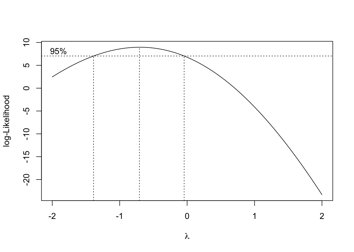

#find lambda
bc$x[which.max(bc$y)]

[1] -0.7070707

• The \(\lambda\) that corresponding to the largest log-likelihood is -0.7070707.
• The optimal choice of power transformation is near \(\lambda\) = -0.71.
• The 95% confidence interval for \(\lambda\) can also be viewed on the graph.
• For easy interpration, we typically use one of -1(\(1/Y\)), 0(\(ln Y\)), 0.5 (\(\sqrt{Y}\)) and 2 (\(Y^2\)) nearest to the optimum. So in this problem, we would choose \(\lambda =-1\). In other words, instead of fitting \(Y\), we use \(Y^{-1}=1/Y\).

Addressing Violations of the Normality Assumption

fit2=lm(1/MPG.highway~Weight)
plot(fit2,which=2)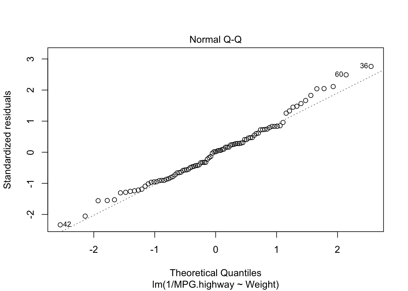

par(mfrow=c(1,2))
plot(fit,which=2)
plot(fit2,which=2)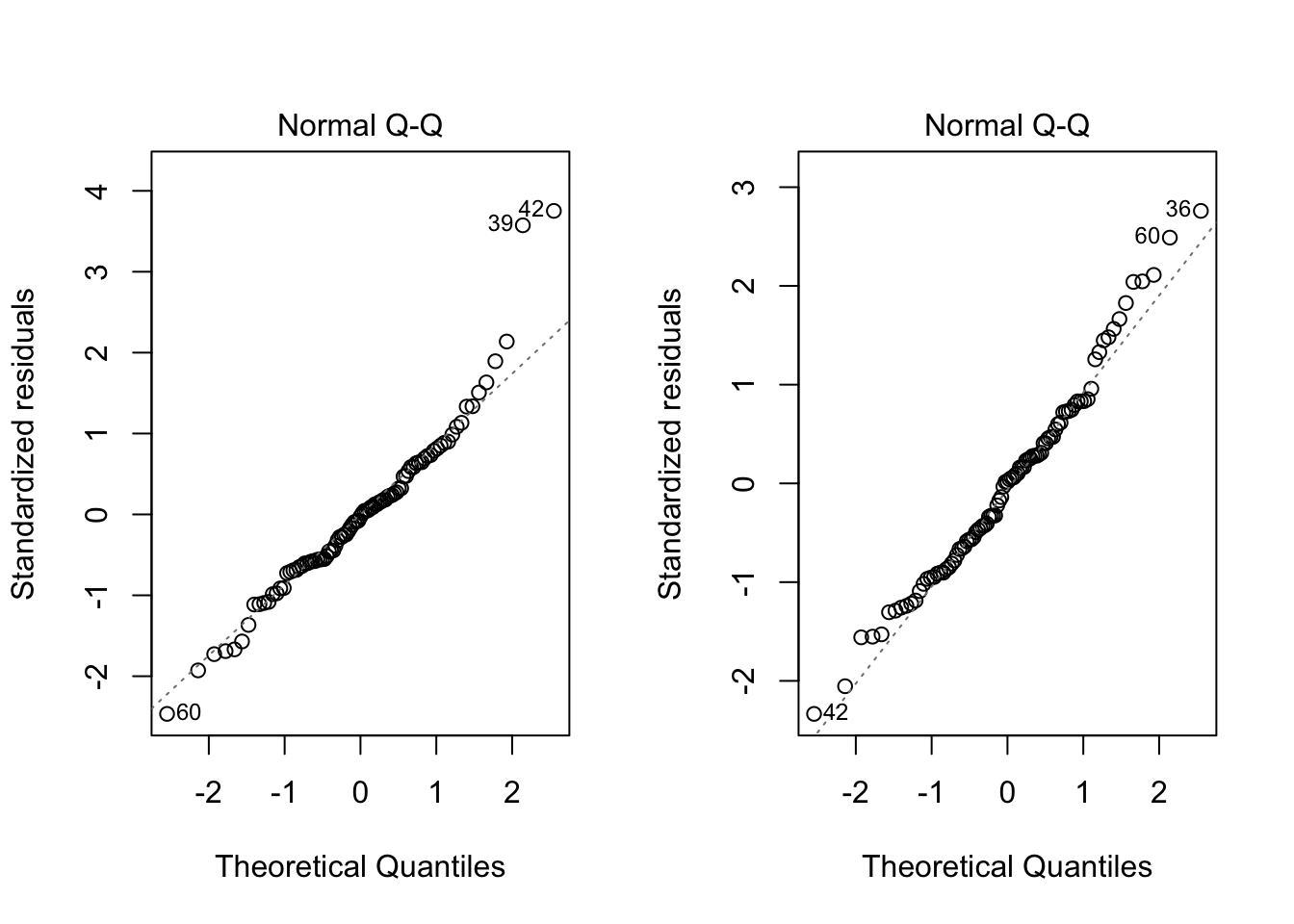

shapiro.test(fit$residuals) #before

    Shapiro-Wilk normality test

data:  fit$residuals
W = 0.95223, p-value = 0.001875

shapiro.test(fit2$residuals) #after 

    Shapiro-Wilk normality test

data:  fit2$residuals
W = 0.98304, p-value = 0.2707

Both the graphical check above and the Shapiro-Wilk test shows the violation of the normality assumption before has been solved. Based on the test result, since the p-value is 0.2707, we can conclude the residuals follow a normal distribution.

Addressing Violations of the Constant Variance Assumption}

library(zoo)

Attaching package: 'zoo'

The following objects are masked from 'package:base':

    as.Date, as.Date.numeric

library(lmtest)

par(mfrow=c(1,2))
plot(fit, which=3)
plot(fit2,which=3)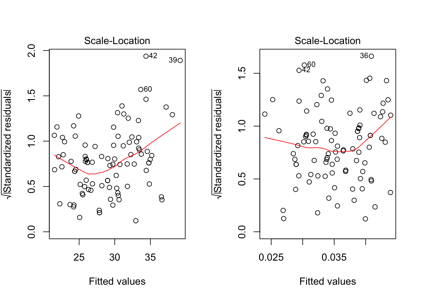 

bptest(MPG.highway~Weight)

    studentized Breusch-Pagan test

data:  MPG.highway ~ Weight
BP = 11.495, df = 1, p-value = 0.0006977

bptest(1/MPG.highway~Weight)

    studentized Breusch-Pagan test

data:  1/MPG.highway ~ Weight
BP = 0.4515, df = 1, p-value = 0.5016

Doing the diagnostic check for constant variance, the graphical check shows the non-constant variance situation has been modified. The BP test also shows the residuals have constanct variance (p-value 0.5016). Sometimes problems of non-normality and non-constant variance go hand-in-hand, so treating one problem frequently cures the other. However, this is not always the case.

Practical Suggestions

• If both constant variance assumption and normality assumption are violated, then try a power transformation on \(Y\) by Box-Cox method.
• If the normality assumption is met, but constant variance assumption is not met, use \(\sqrt{Y}\) or \(log Y\).
• The log transformation (more frequently used) would be more appropriate for more severe cases.
• If 1 and 2 do not work, we need more advanced technique such as Weighted least squares (WLS) regression (Chap 11).

Some notes

\[ \frac{1}{Y}=\beta_0+\beta_1X+\epsilon, \] where \(Y\) is highway mpg and \(X\) is car weight.

• Regression coefficients will need to be interpreted with respect to the transformed scale.

• \(\beta_0\) is the true mean of the reciprocal of highway mpg at \(X=0\) (meaningless in this problem context)

• \(\beta_1\) is the change in the true mean of the reciprocal of highway mpg as a car weight increases by 1 pound.

• There is no straightforward way of “untransforming” them to values that can interpreted in the original scale.

• Even if you transform the response, you can express model predictions back in the original scale.

• This is simply a matter of “untransforming” by using the inverse function of the original transformation.

For example, we want to find a 95% PI for a car weighing 2000 lb.

pred=predict(fit2,newdata=data.frame(Weight=2000),int="prediction",level=0.95)
pred

         fit        lwr        upr
1 0.02652034 0.01973904 0.03330164

1/pred

       fit      lwr      upr
1 37.70691 50.66102 30.02855

• We are 95% confident that the true highway mpg for an unobserved individual car weighing 2000 lb is somewhere between 30.03 to 50.66 miles per gallon.

• The lower and upper prediction limits in R are switched because of the reciprocal transformation we used.

Boxcox Transformation When Response Not Positive

• If the reponses are not strictly postive, then add a constant number to reponses first and the use the Box-Cox method. \[ (Y+\lambda_2)^{\lambda_1} \]

\[ \begin{eqnarray*} t_{\lambda_1,\lambda_2}(Y)=\left \{\begin{array}{ll} \frac{(Y+\lambda_2)^{\lambda_1}-1}{\lambda_1} & \mbox{for } \lambda_1 \neq 0\\ ln (Y+\lambda_2)& \mbox{for } \lambda_1=0\\ \end{array} \right. \end{eqnarray*} \]

Session information

sessionInfo()

R version 3.6.1 (2019-07-05)
Platform: x86_64-apple-darwin15.6.0 (64-bit)
Running under: macOS Mojave 10.14.6

Matrix products: default
BLAS:   /Library/Frameworks/R.framework/Versions/3.6/Resources/lib/libRblas.0.dylib
LAPACK: /Library/Frameworks/R.framework/Versions/3.6/Resources/lib/libRlapack.dylib

locale:
[1] en_US.UTF-8/en_US.UTF-8/en_US.UTF-8/C/en_US.UTF-8/en_US.UTF-8

attached base packages:
[1] stats     graphics  grDevices utils     datasets  methods   base     

other attached packages:
[1] lmtest_0.9-37 zoo_1.8-6     MASS_7.3-51.4

loaded via a namespace (and not attached):
 [1] workflowr_1.4.0 Rcpp_1.0.2      lattice_0.20-38 digest_0.6.20  
 [5] rprojroot_1.3-2 grid_3.6.1      backports_1.1.4 git2r_0.26.1   
 [9] magrittr_1.5    evaluate_0.14   stringi_1.4.3   fs_1.3.1       
[13] whisker_0.3-2   rmarkdown_1.15  tools_3.6.1     stringr_1.4.0  
[17] glue_1.3.1      xfun_0.9        yaml_2.2.0      compiler_3.6.1 
[21] htmltools_0.3.6 knitr_1.24