Detecting hidden heterogeneity in single cell RNA-Seq data

Install packages
Load packages
Load the islet single cell RNA-Seq data
Extract alpha cells (GCG expressed cells) from non-diabetics
Normalization using SCnorm
Calculate the number of detected genes
Run IA-SVA
Find marker genes for the detected heterogeneity (SV2).
Run tSNE to detect the hidden heterogeneity.
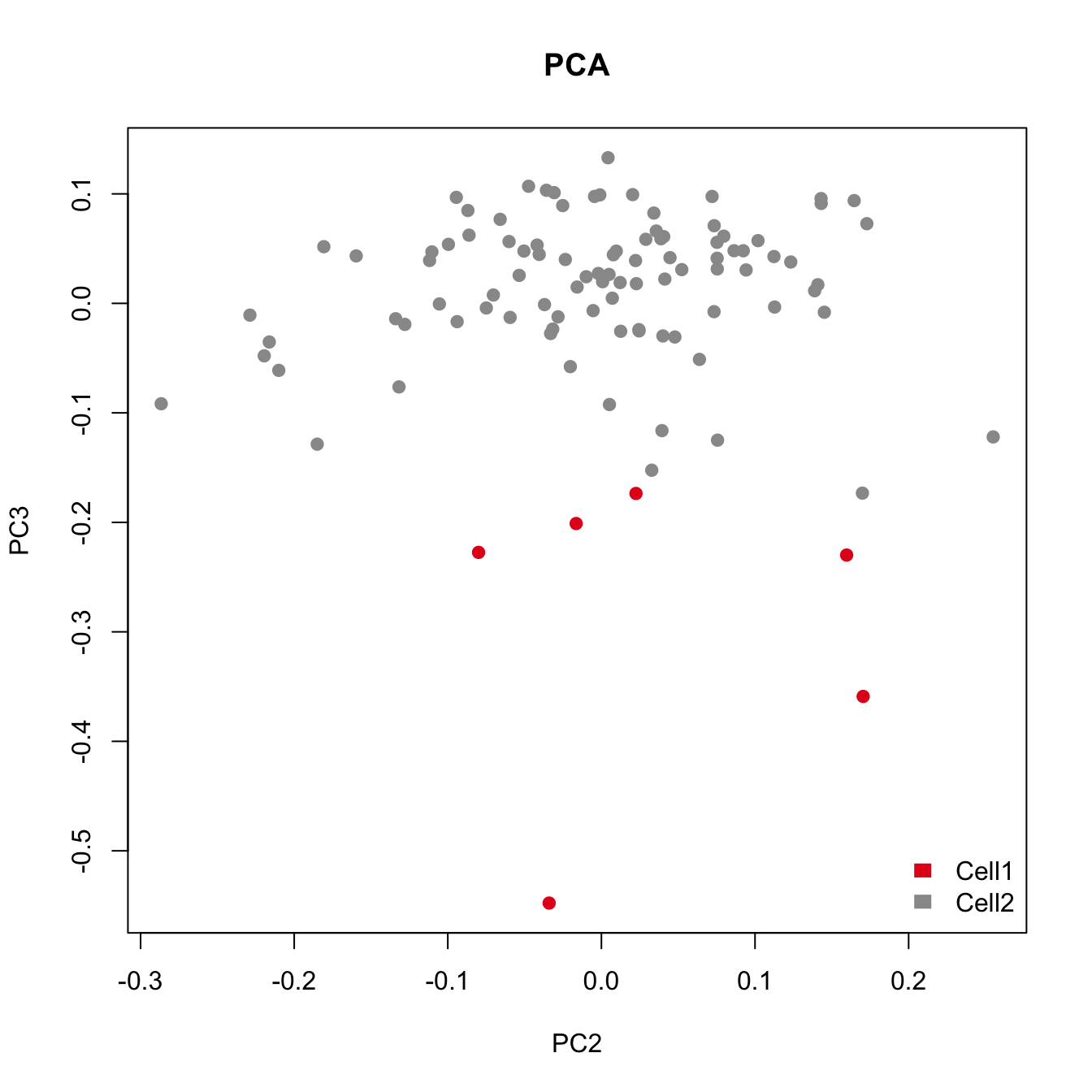
Run principal component analysis (PCA) to detect the hidden heterogeneity (SV2).
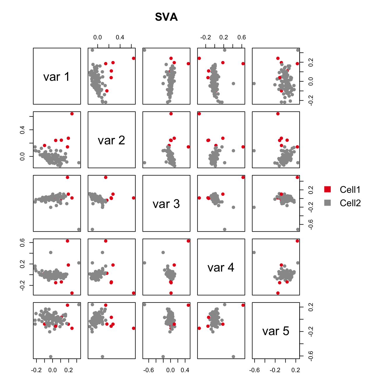
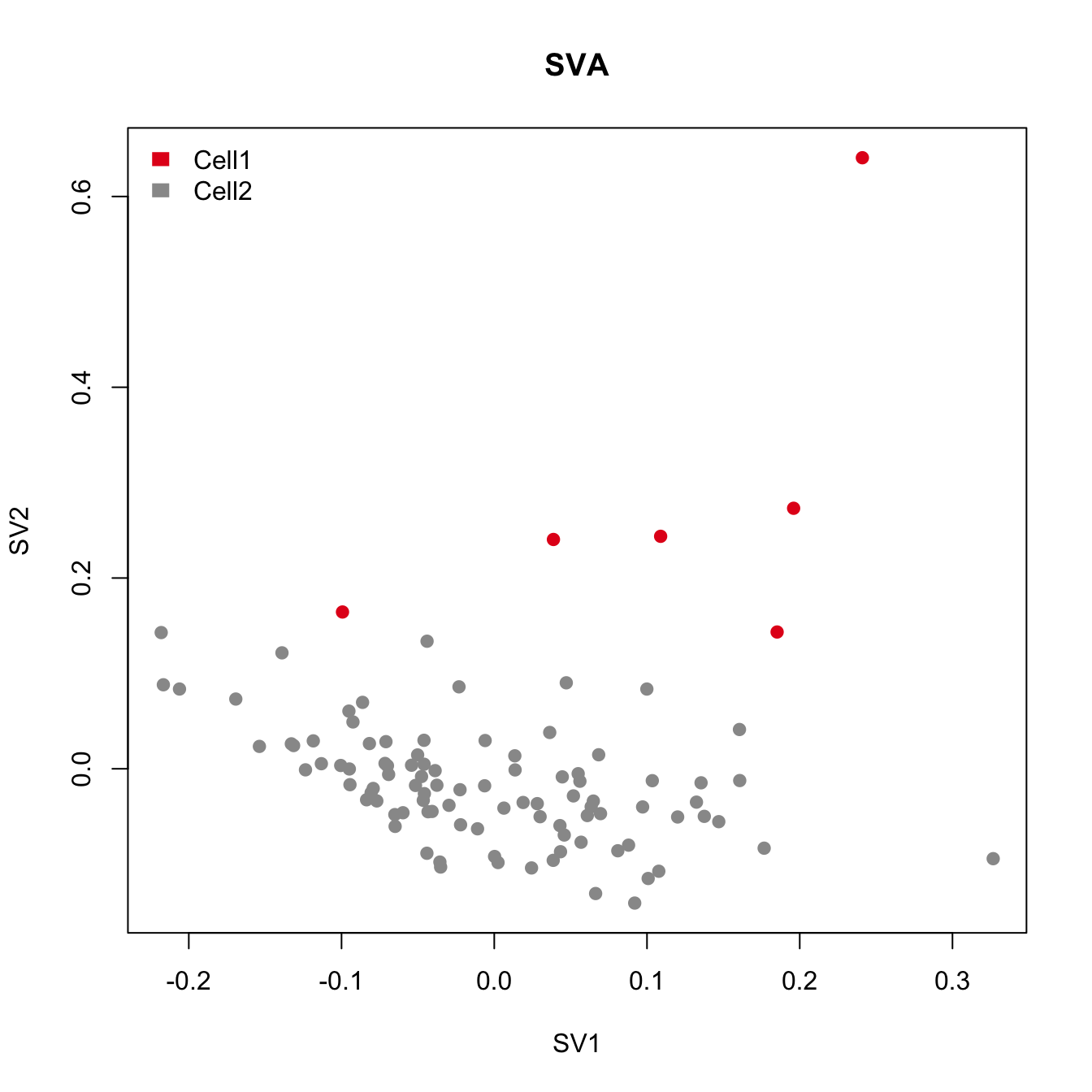
Run surrogate variable analysis (SVA) to detect the hidden heterogeneity (SV2).
Correlation between SV2 and the geometric library size
Session information

Last updated: 2018-08-03

workflowr checks: (Click a bullet for more information)

✔ R Markdown file: up-to-date

Great! Since the R Markdown file has been committed to the Git repository, you know the exact version of the code that produced these results.
✔ Environment: empty

Great job! The global environment was empty. Objects defined in the global environment can affect the analysis in your R Markdown file in unknown ways. For reproduciblity it’s best to always run the code in an empty environment.
✔ Seed: set.seed(20180731)

The command set.seed(20180731) was run prior to running the code in the R Markdown file. Setting a seed ensures that any results that rely on randomness, e.g. subsampling or permutations, are reproducible.
✔ Session information: recorded

Great job! Recording the operating system, R version, and package versions is critical for reproducibility.

✔ Repository version: 6e130ac

Great! You are using Git for version control. Tracking code development and connecting the code version to the results is critical for reproducibility. The version displayed above was the version of the Git repository at the time these results were generated.

Note that you need to be careful to ensure that all relevant files for the analysis have been committed to Git prior to generating the results (you can use wflow_publish or wflow_git_commit). workflowr only checks the R Markdown file, but you know if there are other scripts or data files that it depends on. Below is the status of the Git repository when the results were generated:


Ignored files:
    Ignored:    .DS_Store
    Ignored:    .Rhistory
    Ignored:    .Rproj.user/
    Ignored:    data/.DS_Store
    Ignored:    inst/.DS_Store
    Ignored:    inst/doc/.DS_Store
    Ignored:    vignettes/.DS_Store

Untracked files:
    Untracked:  analysis/figure/
    Untracked:  analysis/hidden_heterogeneity_glioblastoma.Rmd
    Untracked:  output/Lawlor_Islets_Alpha_Doublets_Figure2_ABCD.pdf
    Untracked:  output/Lawlor_Islets_Alpha_Doublets_SV2_Genes_rsqcutoff0.3.txt
    Untracked:  output/Lawlor_Islets_Alpha_Doublets_SV2_Genes_rsqcutoff0.6.txt
    Untracked:  output/Lawlor_Islets_Alpha_iasva_SV2Markers_rsqcutoff0.3_pheatmap_iasvaV0.95.pdf
    Untracked:  output/Lawlor_Islets_Alpha_iasva_SV2Markers_rsqcutoff0.6_pheatmap_iasvaV0.95.pdf

Unstaged changes:
    Deleted:    analysis/about.Rmd
    Modified:   analysis/license.Rmd
    Modified:   output/Clustering_analyses_figure2.pdf

Note that any generated files, e.g. HTML, png, CSS, etc., are not included in this status report because it is ok for generated content to have uncommitted changes.

Expand here to see past versions:

File	Version	Author	Date	Message
Rmd	6e130ac	dleelab	2018-08-03	SCnorm codes updated
Rmd	13e8676	dleelab	2018-08-03	figure size updated
html	c241b04	dleelab	2018-08-03	added
Rmd	bae72f7	dleelab	2018-08-01	figure updated

The iasva package can be used to detect hidden heterogenity within bulk or single cell sequencing data. To illustrate how to use the iasva package for heterogenity detection, we use real-world single cell RNA sequencing (scRNA-Seq) data obtained from human pancreatic islet samples (Lawlor et. al., 2016). This dataset is included in a R data package (“iasvaExamples”) containing data examples for IA-SVA (https://github.com/dleelab/iasvaExamples). To install the package, follow the instruction provided in the GitHub page.

Install packages

#devtools
library(devtools)
#iasva
devtools::install_github("UcarLab/iasva")
#iasvaExamples  
devtools::install_github("dleelab/iasvaExamples")

Load packages

rm(list=ls())
library(irlba) # partial SVD, the augmented implicitly restarted Lanczos bidiagonalization algorithm
library(iasva)
library(iasvaExamples)
library(sva)
library(SCnorm)

Warning: package 'SCnorm' was built under R version 3.5.1

library(Rtsne)
library(pheatmap)
library(corrplot)
library(DescTools) #pcc i.e., Pearson's contingency coefficient
library(RColorBrewer)
library(SummarizedExperiment)

color.vec <- brewer.pal(9, "Set1")[c(1,9)]

# Normalization.
normalize <- function(counts) 
{
    normfactor <- colSums(counts)
    return(t(t(counts)/normfactor)*median(normfactor))
}

Load the islet single cell RNA-Seq data

data("Lawlor_Islet_scRNAseq_Read_Counts")
data("Lawlor_Islet_scRNAseq_Annotations")
ls()

[1] "color.vec"                         "Lawlor_Islet_scRNAseq_Annotations"
[3] "Lawlor_Islet_scRNAseq_Read_Counts" "normalize"

counts <- Lawlor_Islet_scRNAseq_Read_Counts
anns <- Lawlor_Islet_scRNAseq_Annotations
dim(anns)

[1] 638  26

dim(counts)

[1] 26542   638

summary(anns)

     run             cell.type             COL1A1          INS       
 Length:638         Length:638         Min.   :1.00   Min.   :1.000  
 Class :character   Class :character   1st Qu.:1.00   1st Qu.:1.000  
 Mode  :character   Mode  :character   Median :1.00   Median :1.000  
                                       Mean   :1.03   Mean   :1.414  
                                       3rd Qu.:1.00   3rd Qu.:2.000  
                                       Max.   :2.00   Max.   :2.000  
                                                                     
     PRSS1            SST             GCG            KRT19      
 Min.   :1.000   Min.   :1.000   Min.   :1.000   Min.   :1.000  
 1st Qu.:1.000   1st Qu.:1.000   1st Qu.:1.000   1st Qu.:1.000  
 Median :1.000   Median :1.000   Median :1.000   Median :1.000  
 Mean   :1.038   Mean   :1.039   Mean   :1.375   Mean   :1.044  
 3rd Qu.:1.000   3rd Qu.:1.000   3rd Qu.:2.000   3rd Qu.:1.000  
 Max.   :2.000   Max.   :2.000   Max.   :2.000   Max.   :2.000  
                                                                
      PPY          num.genes             Cell_ID        UNOS_ID   
 Min.   :1.000   Min.   :3529   10th_C1_S59  :  1   ACCG268 :136  
 1st Qu.:1.000   1st Qu.:5270   10th_C10_S104:  1   ACJV399 :108  
 Median :1.000   Median :6009   10th_C11_S96 :  1   ACEL337 :103  
 Mean   :1.028   Mean   :5981   10th_C13_S61 :  1   ACIW009 : 93  
 3rd Qu.:1.000   3rd Qu.:6676   10th_C14_S53 :  1   ACCR015A: 57  
 Max.   :2.000   Max.   :8451   10th_C16_S105:  1   ACIB065 : 57  
                                (Other)      :632   (Other) : 84  
      Age        Biomaterial_Provider    Gender              Phenotype  
 Min.   :22.00   IIDP      : 45       Female:303   Non-Diabetic   :380  
 1st Qu.:29.00   Prodo Labs:593       Male  :335   Type 2 Diabetic:258  
 Median :42.00                                                          
 Mean   :39.63                                                          
 3rd Qu.:53.00                                                          
 Max.   :56.00                                                          
                                                                        
               Race          BMI          Cell_Type     Patient_ID 
 African American:175   Min.   :22.00   INS    :264   P1     :136  
 Hispanic        :165   1st Qu.:26.60   GCG    :239   P8     :108  
 White           :298   Median :32.95   KRT19  : 28   P3     :103  
                        Mean   :32.85   SST    : 25   P7     : 93  
                        3rd Qu.:35.80   PRSS1  : 24   P5     : 57  
                        Max.   :55.00   none   : 21   P6     : 57  
                                        (Other): 37   (Other): 84  
 Sequencing_Run Batch       Coverage       Percent_Aligned 
 12t    : 57    B1:193   Min.   :1206135   Min.   :0.8416  
 4th    : 57    B2:148   1st Qu.:2431604   1st Qu.:0.8769  
 9th    : 57    B3:297   Median :3042800   Median :0.8898  
 10t    : 56             Mean   :3160508   Mean   :0.8933  
 7th    : 55             3rd Qu.:3871697   3rd Qu.:0.9067  
 3rd    : 53             Max.   :5931638   Max.   :0.9604  
 (Other):303                                               
 Mitochondrial_Fraction Num_Expressed_Genes
 Min.   :0.003873       Min.   :3529       
 1st Qu.:0.050238       1st Qu.:5270       
 Median :0.091907       Median :6009       
 Mean   :0.108467       Mean   :5981       
 3rd Qu.:0.142791       3rd Qu.:6676       
 Max.   :0.722345       Max.   :8451

ContCoef(table(anns$Gender, anns$Cell_Type))

[1] 0.225969

ContCoef(table(anns$Phenotype, anns$Cell_Type))

[1] 0.1145096

ContCoef(table(anns$Race, anns$Cell_Type))

[1] 0.3084146

ContCoef(table(anns$Patient_ID, anns$Cell_Type))

[1] 0.5232058

ContCoef(table(anns$Batch, anns$Cell_Type))

[1] 0.3295619

The annotations describing the islet samples and experimental settings are stored in “anns” and the read counts information is stored in “counts”.

Extract alpha cells (GCG expressed cells) from non-diabetics

To illustrate how IA-SVA can be used to detect hidden heterogeneity within a homogenous cell population (i.e., alpha cells), we use read counts of alpha cells from healthy (non-diabetic) subjects (n = 101).

# Selected T2D patients/GCG cell type
counts <- counts[, (anns$Phenotype!="Non-Diabetic")&(anns$Cell_Type=="GCG")]
anns <- subset(anns, (Phenotype!="Non-Diabetic")&(Cell_Type=="GCG"))
dim(counts)

[1] 26542 101

dim(anns)

[1] 101 26

anns <- droplevels(anns)
prop.zeros <- sum(counts==0)/length(counts)
prop.zeros

[1] 0.6952497

# filter out genes that are sparsely and lowly expressed
filter = apply(counts, 1, function(x) length(x[x>5])>=3)
counts = counts[filter,]
dim(counts)

[1] 14384 101

prop.zeros <- sum(counts==0)/length(counts)
prop.zeros

[1] 0.4520968

Normalization using SCnorm

## count-depth relationship for all genes
Conditions = rep(c(1), each=101)
countDeptEst <- plotCountDepth(Data = counts, Conditions = Conditions,
                               FilterCellProportion = .1, NCores=8)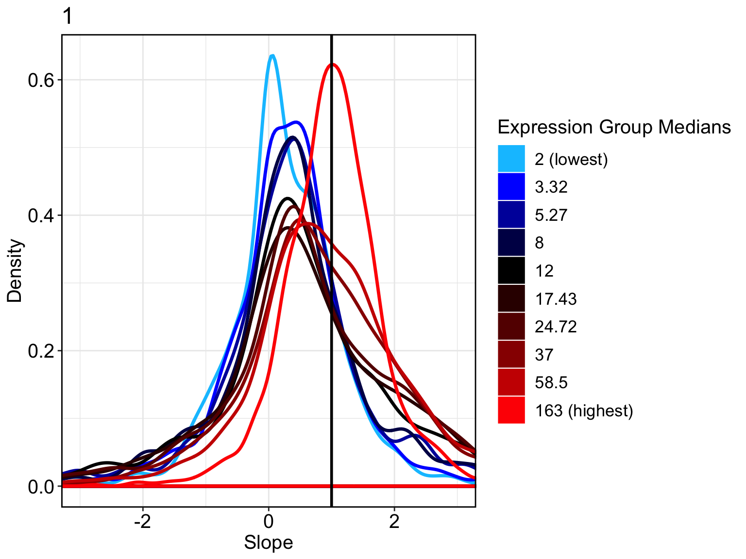

DataNorm <- SCnorm(Data = counts, Conditions = Conditions,
                   PrintProgressPlots = FALSE,
                   FilterCellNum = 10,
                   NCores=8)

Setting up parallel computation using 8 cores

Gene filter is applied within each condition.

1223 genes in condition 1 will not be included in the normalization due to 
             the specified filter criteria.

A list of these genes can be accessed in output, 
    see vignette for example.

Finding K for Condition 1

Trying K = 1

Trying K = 2

Trying K = 3

Trying K = 4

Trying K = 5

Trying K = 6

Trying K = 7

Trying K = 8

Done!

counts <- SingleCellExperiment::normcounts(DataNorm)
summary(colSums(counts))

   Min. 1st Qu.  Median    Mean 3rd Qu.    Max. 
1274488 1315313 1332682 1358957 1386293 1650415

Calculate the number of detected genes

It is well known that the number of detected genes in each cell explains a very large portion of variability in scRNA-Seq data (Hicks et. al. 2015 BioRxiv, McDavid et. al. 2016 Nature Biotechnology). Frequently, the first principal component of log-transformed scRNA-Seq read counts is highly correlated with the number of detected genes (e.g., r > 0.9). Here, we calculate the number of detected genes for islet cells, which will be used as an known factor in the IA-SVA analyses.

Num_Detected_Genes <- colSums(counts>0)
Geo_Lib <- colSums(log(counts+1))
summary(Num_Detected_Genes)

   Min. 1st Qu.  Median    Mean 3rd Qu.    Max. 
   5787    7043    7925    7881    8652   10188

summary(Geo_Lib)

   Min. 1st Qu.  Median    Mean 3rd Qu.    Max. 
  16571   20527   24507   24349   27475   33830

barplot(Num_Detected_Genes, xlab="Cell", las=2,
        ylab = "Number of detected genes")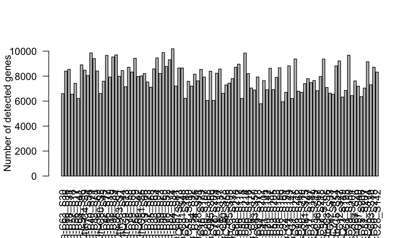

lcounts <- log(counts + 1)

# PC1 and Geometric library size correlation
pc1 = irlba(lcounts - rowMeans(lcounts), 1)$v[,1] ## partial SVD
cor(Num_Detected_Genes, pc1)

[1] 0.9778019

cor(Geo_Lib, pc1)

[1] 0.99461

Run IA-SVA

Here, we run IA-SVA using Patient_ID and Geo_Lib_Size as known factors and identify five hidden factors. SVs are plotted in a pairwise fashion to uncover which SVs can seperate cell types.

set.seed(4543535)
Patient_ID <- anns$Patient_ID
mod <- model.matrix(~Patient_ID+Geo_Lib)
summ_exp <- SummarizedExperiment(assays = counts)
iasva.res<- iasva(summ_exp, mod[,-1],verbose=FALSE, permute=FALSE, num.sv=5) ##irlba

IA-SVA running...


SV 1 Detected!


SV 2 Detected!


SV 3 Detected!


SV 4 Detected!


SV 5 Detected!


# of significant surrogate variables: 5

iasva.sv <- iasva.res$sv
plot(iasva.sv[,1], iasva.sv[,2], xlab="SV1", ylab="SV2")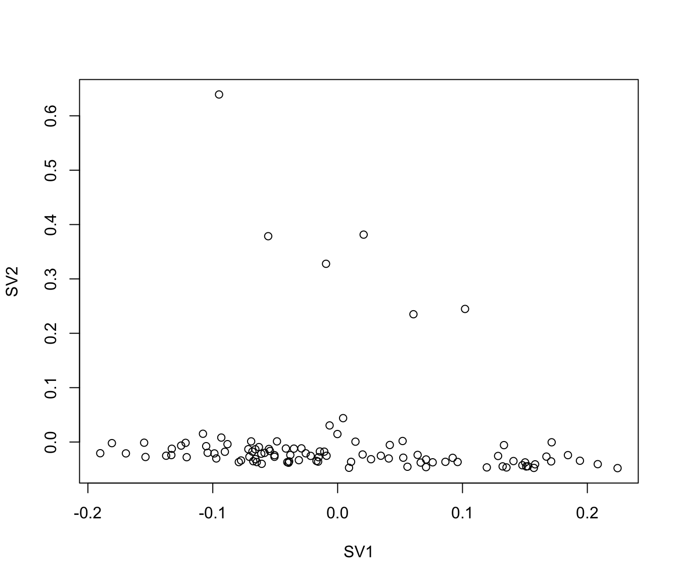

Cluster <- as.factor(iasva.sv[,2] < 0.1) 
levels(Cluster)=c("Cell1","Cell2")
table(Cluster)

Cluster
Cell1 Cell2 
    6    95

# We identified 6 outlier cells based on SV2 that are marked in red
pairs(iasva.sv, main="IA-SVA", pch=21, col=color.vec[Cluster],
      bg=color.vec[Cluster], oma=c(4,4,6,12)) #4,4,6,12
legend("right", levels(Cluster), fill=color.vec, bty="n")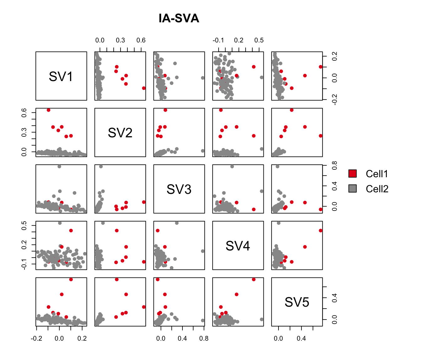

plot(iasva.sv[,1:2], main="IA-SVA", pch=21, xlab="SV1", ylab="SV2",
     col=color.vec[Cluster], bg=color.vec[Cluster])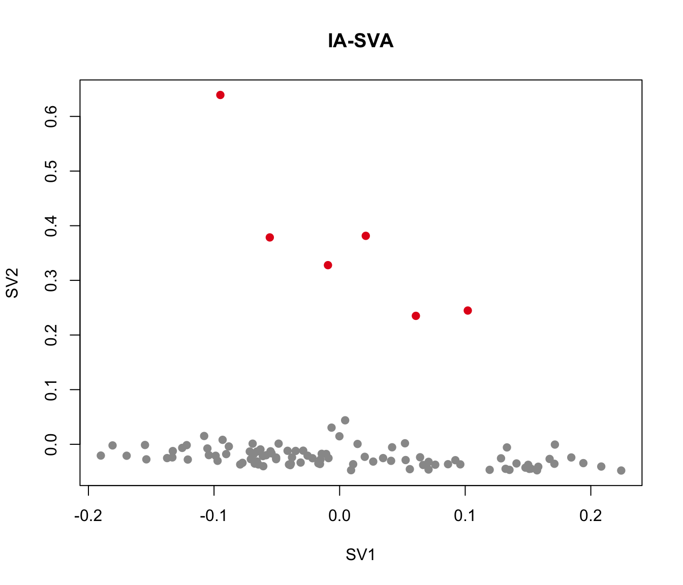

cor(Num_Detected_Genes, iasva.sv[,2])

[1] 0.1571675

cor(Geo_Lib, iasva.sv[,2])

[1] 0.2009796

corrplot(cor(iasva.sv))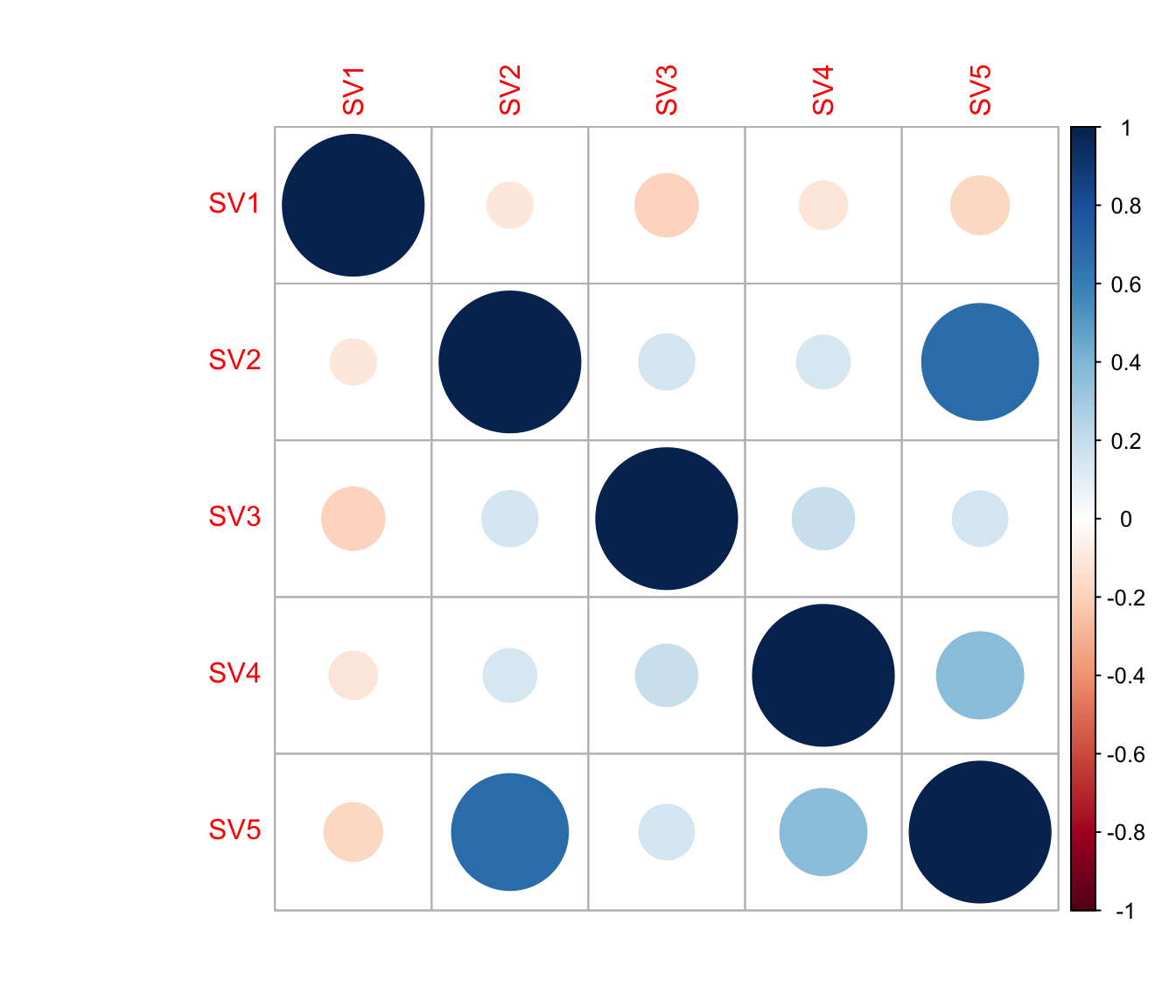

As shown in the above figure, SV2 clearly separates alpha cells into two groups: 6 outlier cells (marked in red) and the rest of the alpha cells (marked in green). SV3 and SV4 also capture outlier cells. However, we will focus on SV2 in the rest of the analyses.

Find marker genes for the detected heterogeneity (SV2).

Here, using the find_markers() function we find marker genes (n=105 genes) that are significantly associated with SV2 (multiple testing adjusted p-value < 0.05, default significance cutoff, and R-squared value > 0.3, default R-squared cutoff).

# try different R2 thresholds
pdf("output/Clustering_analyses_figure2.pdf")
r2.results <- study_R2(summ_exp, iasva.sv, selected.svs=2, no.clusters=2)

# of markers (): 396

total # of unique markers: 396

# of markers (): 237

total # of unique markers: 237

# of markers (): 177

total # of unique markers: 177

# of markers (): 143

total # of unique markers: 143

# of markers (): 108

total # of unique markers: 108

# of markers (): 93

total # of unique markers: 93

# of markers (): 72

total # of unique markers: 72

# of markers (): 58

total # of unique markers: 58

# of markers (): 47

total # of unique markers: 47

# of markers (): 35

total # of unique markers: 35

# of markers (): 27

total # of unique markers: 27

# of markers (): 22

total # of unique markers: 22

# of markers (): 12

total # of unique markers: 12

# of markers (): 8

total # of unique markers: 8

# of markers (): 4

total # of unique markers: 4

# of markers (): 2

total # of unique markers: 2

# of markers (): 1

total # of unique markers: 1

dev.off()

quartz_off_screen 
                2

marker.counts <- find_markers(summ_exp, as.matrix(iasva.sv[,2]), rsq.cutoff = 0.6)

# of markers (): 27

total # of unique markers: 27

marker.counts.long <- find_markers(summ_exp, as.matrix(iasva.sv[,2]), rsq.cutoff = 0.3)

# of markers (): 108

total # of unique markers: 108

nrow(marker.counts)

[1] 27

rownames(marker.counts)

 [1] "PMEPA1"      "LINC00152"   "MIR4435-1HG" "ENG"         "ITGA5"      
 [6] "TMEM233"     "PRDM1"       "C8orf4"      "ERG"         "THBS1"      
[11] "MEF2C"       "LGALS1"      "CD93"        "ELTD1"       "COL4A1"     
[16] "COL4A2"      "HBEGF"       "SPARC"       "SPARCL1"     "RAPGEF5"    
[21] "KDR"         "GNG11"       "CD9"         "PODXL"       "PLVAP"      
[26] "IFI16"       "RHOJ"

nrow(marker.counts.long)

[1] 108

anno.col <- data.frame(Cluster=Cluster, SV2=iasva.sv[,2])
rownames(anno.col) <- colnames(marker.counts)
head(anno.col)

            Cluster         SV2
4th-C63_S30   Cell2 -0.02724532
4th-C66_S36   Cell2 -0.02091476
4th-C18_S31   Cell2 -0.01190674
4th-C57_S18   Cell1  0.23502845
4th-C56_S17   Cell2 -0.03704850
4th-C68_S41   Cell2 -0.03570599

cluster.col <- color.vec[1:2]
names(cluster.col) <- as.vector(levels(Cluster))
anno.colors <- list(Cluster=cluster.col)
anno.colors

$Cluster
    Cell1     Cell2 
"#E41A1C" "#999999"

pheatmap(log(marker.counts+1), show_colnames =FALSE, 
         clustering_method = "ward.D2",cutree_cols = 2,annotation_col = anno.col,
         annotation_colors = anno.colors)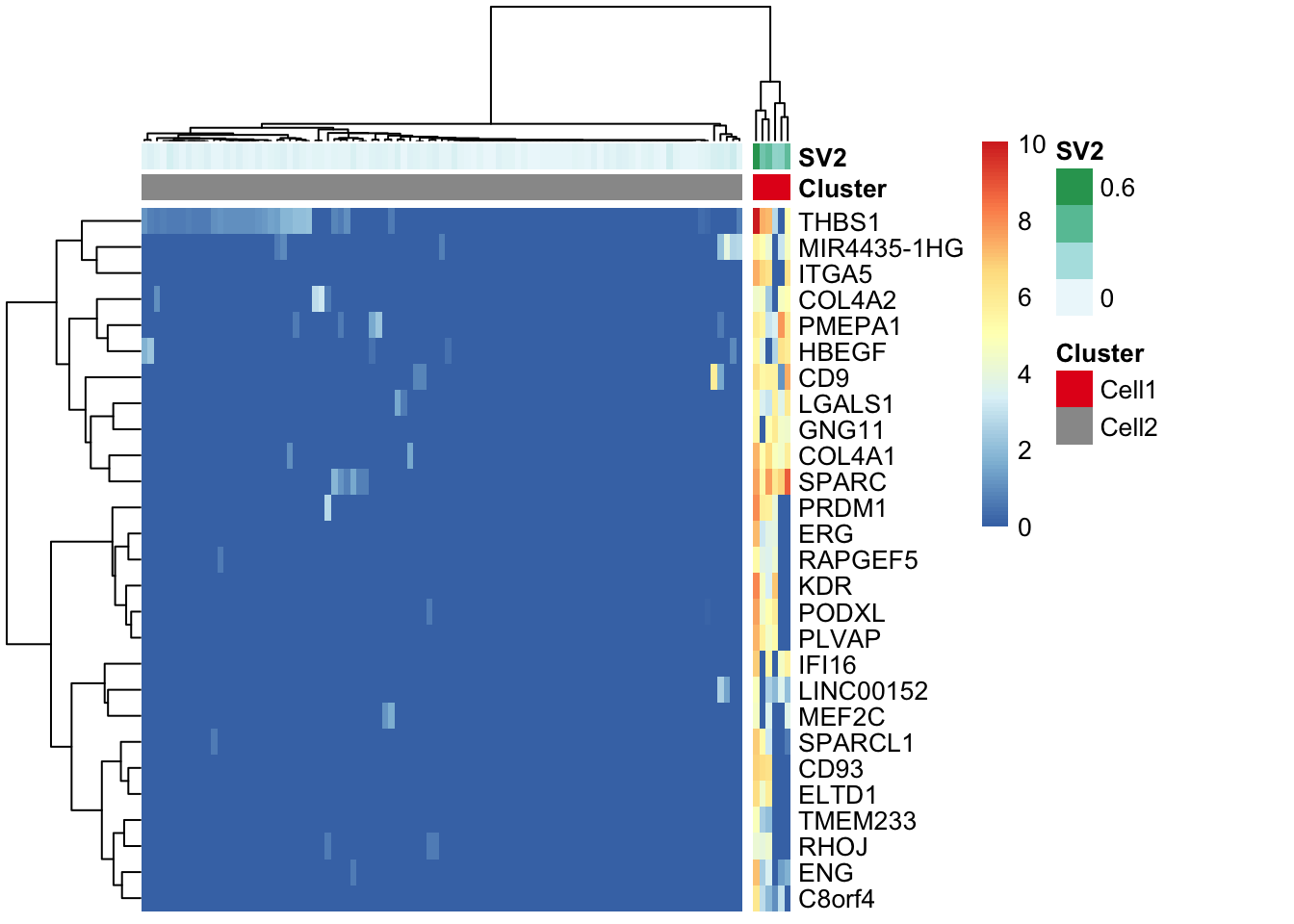

Run tSNE to detect the hidden heterogeneity.

For comparison purposes, we applied tSNE on read counts of all genes to identify the hidden heterogeneity. We used the Rtsne R package with default settings.

set.seed(323542534)
tsne.res <- Rtsne(t(lcounts), dims = 2)
plot(tsne.res$Y, main="tSNE", xlab="tSNE Dim1", ylab="tSNE Dim2", pch=21, 
     col=color.vec[Cluster], bg=color.vec[Cluster], oma=c(4,4,6,12))
legend("bottomright", levels(Cluster), border="white", fill=color.vec, bty="n")

As shown above, tSNE fails to detect the outlier cells that are identified by IA-SVA when all genes are used. Same color coding is used as above.

Run principal component analysis (PCA) to detect the hidden heterogeneity (SV2).

Here, we use PCA to detect the hidden heterogeneity (SV2) detected by IA-SVA.

set.seed(345233)
pca.res = irlba(lcounts - rowMeans(lcounts), 5)$v ## partial SVD

pairs(pca.res, main="PCA", pch=21, col=color.vec[Cluster],
      bg=color.vec[Cluster], oma=c(4,4,6,12)) #4,4,6,12
legend("right", levels(Cluster), border="white", fill=color.vec, bty="n")

plot(pca.res[,2:3], main="PCA", xlab="PC2", ylab="PC3", pch=21,
     col=color.vec[Cluster], bg=color.vec[Cluster], oma=c(4,4,6,12))
legend("bottomright", levels(Cluster), border="white", fill=color.vec, bty="n")

PC3 somewhat captures the six outlier cells, however this seperation is not as clear as the IA-SVA results.

Run surrogate variable analysis (SVA) to detect the hidden heterogeneity (SV2).

Here, for comparison purposes we use SVA (using thre SVs) to detect the hidden heterogeneity in our example data.

mod1 <- model.matrix(~Patient_ID+Geo_Lib)
mod0 <- cbind(mod1[,1])
sva.res = svaseq(counts,mod1,mod0, n.sv=5)$sv

Number of significant surrogate variables is:  5 
Iteration (out of 5 ):1  2  3  4  5

pairs(sva.res, main="SVA", pch=21, col=color.vec[Cluster], bg=color.vec[Cluster], oma=c(4,4,6,12)) #4,4,6,12
legend("right", levels(Cluster), border="white", fill=color.vec, bty="n")

plot(sva.res[,1:2], main="SVA", xlab="SV1", ylab="SV2", pch=21, col=color.vec[Cluster], bg=color.vec[Cluster])
legend("topleft", levels(Cluster), border="white", fill=color.vec, bty="n")

SV2 is associated with the six outlier samples, however the seperation of these cells is not as clear as the IA-SVA results.

Correlation between SV2 and the geometric library size

cor(Num_Detected_Genes, iasva.sv[,2])

[1] 0.1571675

cor(Geo_Lib, iasva.sv[,2])

[1] 0.2009796

pdf(file="output/Lawlor_Islets_Alpha_Doublets_Figure2_ABCD.pdf", width=5, height=6)
layout(matrix(c(1,2,3,4), nrow=2, ncol=2, byrow=TRUE))
plot(iasva.sv[,1:2], main="IA-SVA", pch=21, xlab="SV1", ylab="SV2", col=color.vec[Cluster], bg=color.vec[Cluster])
legend("topright", levels(Cluster), border="white", fill=color.vec, bty="n")
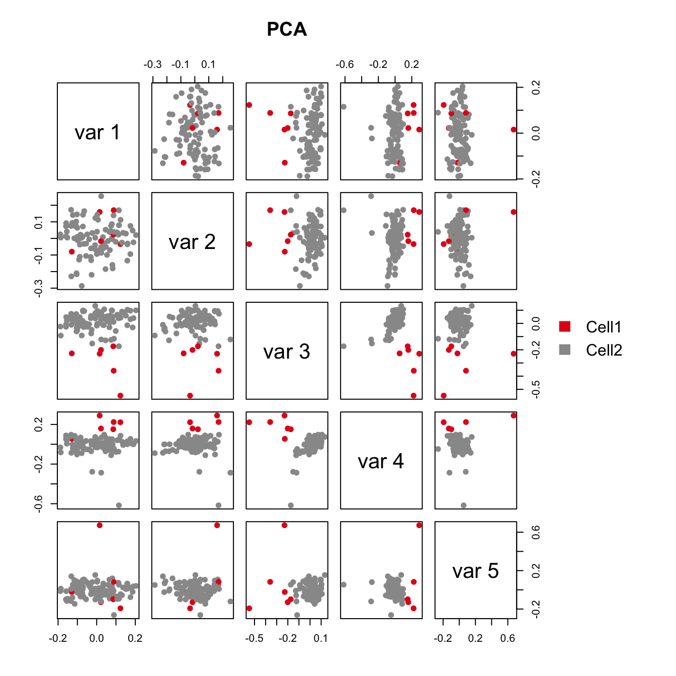
plot(pca.res[,2:3], main="PCA", pch=21, xlab="PC2", ylab="PC3", col=color.vec[Cluster], bg=color.vec[Cluster])
plot(sva.res[,1:2], main="USVA", xlab="SV1", ylab="SV2", pch=21, col=color.vec[Cluster], bg=color.vec[Cluster])
plot(tsne.res$Y, main="tSNE", xlab="Dimension 1", ylab="Dimension 2", pch=21, col=color.vec[Cluster], bg=color.vec[Cluster])
dev.off()

quartz_off_screen 
                2

anno.col <- data.frame(Cluster=Cluster)
rownames(anno.col) <- colnames(marker.counts)
head(anno.col)

            Cluster
4th-C63_S30   Cell2
4th-C66_S36   Cell2
4th-C18_S31   Cell2
4th-C57_S18   Cell1
4th-C56_S17   Cell2
4th-C68_S41   Cell2

cluster.col <- color.vec
names(cluster.col) <- as.vector(levels(Cluster))
anno.colors <- list(Cluster=cluster.col)
anno.colors

$Cluster
    Cell1     Cell2 
"#E41A1C" "#999999"

pheatmap(log(marker.counts+1), show_colnames =FALSE, 
         clustering_method = "ward.D2",cutree_cols = 2,annotation_col = anno.col,
         annotation_colors = anno.colors,
         filename="output/Lawlor_Islets_Alpha_iasva_SV2Markers_rsqcutoff0.6_pheatmap_iasvaV0.95.pdf",
         width=6, height=5)

pheatmap(log(marker.counts.long+1), show_colnames =FALSE,
         clustering_method = "ward.D2",cutree_cols = 2,annotation_col = anno.col,
         annotation_colors = anno.colors,
         filename="output/Lawlor_Islets_Alpha_iasva_SV2Markers_rsqcutoff0.3_pheatmap_iasvaV0.95.pdf",
         width=6, height=14)

write.table(as.data.frame(rownames(marker.counts)),
            file="output/Lawlor_Islets_Alpha_Doublets_SV2_Genes_rsqcutoff0.6.txt", quote=F,
              row.names=F, col.names=F, sep=" ")

write.table(as.data.frame(rownames(marker.counts.long)),
            file="output/Lawlor_Islets_Alpha_Doublets_SV2_Genes_rsqcutoff0.3.txt", quote=F,
              row.names=F, col.names=F, sep=" ")

Session information

sessionInfo()

R version 3.5.0 (2018-04-23)
Platform: x86_64-apple-darwin15.6.0 (64-bit)
Running under: macOS Sierra 10.12.6

Matrix products: default
BLAS: /Library/Frameworks/R.framework/Versions/3.5/Resources/lib/libRblas.0.dylib
LAPACK: /Library/Frameworks/R.framework/Versions/3.5/Resources/lib/libRlapack.dylib

locale:
[1] en_US.UTF-8/en_US.UTF-8/en_US.UTF-8/C/en_US.UTF-8/en_US.UTF-8

attached base packages:
[1] parallel  stats4    stats     graphics  grDevices utils     datasets 
[8] methods   base     

other attached packages:
 [1] SummarizedExperiment_1.10.1 DelayedArray_0.6.1         
 [3] matrixStats_0.53.1          Biobase_2.40.0             
 [5] GenomicRanges_1.32.3        GenomeInfoDb_1.16.0        
 [7] IRanges_2.14.10             S4Vectors_0.18.3           
 [9] BiocGenerics_0.26.0         RColorBrewer_1.1-2         
[11] DescTools_0.99.24           corrplot_0.84              
[13] pheatmap_1.0.10             Rtsne_0.13                 
[15] SCnorm_1.2.1                sva_3.28.0                 
[17] BiocParallel_1.14.2         genefilter_1.62.0          
[19] mgcv_1.8-23                 nlme_3.1-137               
[21] iasvaExamples_1.0.0         iasva_0.99.3               
[23] irlba_2.3.2                 Matrix_1.2-14              
[25] workflowr_1.0.1             rmarkdown_1.9              

loaded via a namespace (and not attached):
 [1] bitops_1.0-6               bit64_0.9-7               
 [3] rprojroot_1.3-2            tools_3.5.0               
 [5] backports_1.1.2            R6_2.2.2                  
 [7] DBI_1.0.0                  lazyeval_0.2.1            
 [9] colorspace_1.3-2           tidyselect_0.2.4          
[11] moments_0.14               bit_1.1-14                
[13] compiler_3.5.0             git2r_0.21.0              
[15] quantreg_5.36              expm_0.999-2              
[17] SparseM_1.77               labeling_0.3              
[19] scales_0.5.0               mvtnorm_1.0-8             
[21] stringr_1.3.1              digest_0.6.15             
[23] foreign_0.8-70             R.utils_2.6.0             
[25] XVector_0.20.0             pkgconfig_2.0.1           
[27] htmltools_0.3.6            manipulate_1.0.1          
[29] limma_3.36.2               rlang_0.2.1               
[31] RSQLite_2.1.1              bindr_0.1.1               
[33] dplyr_0.7.5                R.oo_1.22.0               
[35] RCurl_1.95-4.10            magrittr_1.5              
[37] GenomeInfoDbData_1.1.0     Rcpp_0.12.17              
[39] munsell_0.4.3              R.methodsS3_1.7.1         
[41] stringi_1.2.2              whisker_0.3-2             
[43] yaml_2.1.19                MASS_7.3-50               
[45] zlibbioc_1.26.0            plyr_1.8.4                
[47] grid_3.5.0                 blob_1.1.1                
[49] lattice_0.20-35            splines_3.5.0             
[51] annotate_1.58.0            knitr_1.20                
[53] pillar_1.2.3               boot_1.3-20               
[55] reshape2_1.4.3             XML_3.98-1.11             
[57] glue_1.2.0                 evaluate_0.10.1           
[59] data.table_1.11.4          MatrixModels_0.4-1        
[61] gtable_0.2.0               purrr_0.2.5               
[63] assertthat_0.2.0           ggplot2_2.2.1.9000        
[65] xtable_1.8-2               survival_2.42-3           
[67] SingleCellExperiment_1.2.0 tibble_1.4.2              
[69] AnnotationDbi_1.42.1       memoise_1.1.0             
[71] bindrcpp_0.2.2             cluster_2.0.7-1

This reproducible R Markdown analysis was created with workflowr 1.0.1