Detecting cell-cycle stage difference in glioblastoma cells

Install packages
Load packages
Load the glioblastoma single cell RNA-Seq data
Extract glioblastoma cells from Patient MGH30
Normalization using SCnorm
Calculate the number of detected genes
Run IA-SVA
Find marker genes for the detected heterogeneity (SV1).
Cell type assignment using scran R package
Run tSNE post IA-SVA analyses, i.e., run tSNE on marker genes associated with SV1 as detected by IA-SVA.
Run principal component analysis (PCA) to detect the hidden heterogeneity (SV1).
Run surrogate variable analysis (SVA) to detect the hidden heterogeneity (SV1).
Correlation between SV1 and the geometric library size
Session information

Last updated: 2018-08-03

workflowr checks: (Click a bullet for more information)

✔ R Markdown file: up-to-date

Great! Since the R Markdown file has been committed to the Git repository, you know the exact version of the code that produced these results.
✔ Environment: empty

Great job! The global environment was empty. Objects defined in the global environment can affect the analysis in your R Markdown file in unknown ways. For reproduciblity it’s best to always run the code in an empty environment.
✔ Seed: set.seed(20180731)

The command set.seed(20180731) was run prior to running the code in the R Markdown file. Setting a seed ensures that any results that rely on randomness, e.g. subsampling or permutations, are reproducible.
✔ Session information: recorded

Great job! Recording the operating system, R version, and package versions is critical for reproducibility.
✔ Repository version: 2689835
Great! You are using Git for version control. Tracking code development and connecting the code version to the results is critical for reproducibility. The version displayed above was the version of the Git repository at the time these results were generated.

Note that you need to be careful to ensure that all relevant files for the analysis have been committed to Git prior to generating the results (you can use wflow_publish or wflow_git_commit). workflowr only checks the R Markdown file, but you know if there are other scripts or data files that it depends on. Below is the status of the Git repository when the results were generated:
```
Ignored files:
    Ignored:    .DS_Store
    Ignored:    .Rhistory
    Ignored:    .Rproj.user/
    Ignored:    data/.DS_Store
    Ignored:    inst/.DS_Store
    Ignored:    inst/doc/.DS_Store
    Ignored:    vignettes/.DS_Store

Untracked files:
    Untracked:  analysis/figure/
    Untracked:  output/CC_genes.long.txt
    Untracked:  output/CC_genes.short.txt
    Untracked:  output/Clustering_analyses_figure3_sv1.pdf
    Untracked:  output/Patel_Glioblastoma_MGH30_CellCycle_Figure3ABCD.pdf
    Untracked:  output/Patel_Glioblastoma_MGH30_Cellcycle_SV1_Genes_rsqcutoff0.3.txt
    Untracked:  output/Patel_Glioblastoma_MGH30_Cellcycle_SV1_Genes_rsqcutoff0.4.txt
    Untracked:  output/Patel_Glioblastoma_MGH30_iasva_SV1_genes_rsqcutoff0.3_pheatmap_iasvaV0.95_Figure3F.pdf
```
Note that any generated files, e.g. HTML, png, CSS, etc., are not included in this status report because it is ok for generated content to have uncommitted changes.

Expand here to see past versions:

File	Version	Author	Date	Message
Rmd	2689835	dleelab	2018-08-03	error corrected
Rmd	a414c7c	dleelab	2018-08-03	added
html	c241b04	dleelab	2018-08-03	added

Here, we illustrate how to use the iasva package to detect cell cycle stage difference within single cell RNA sequencing data. We use single cell RNA sequencing (scRNA-Seq) data obtained from human glioblastoma samples (Petel et. al., 2014). This dataset is included in a R data package (“iasvaExamples”) containing data examples for IA-SVA (https://github.com/dleelab/iasvaExamples). To install the package, follow the instruction provided in the GitHub page.

Install packages

#devtools
library(devtools)
#iasva
devtools::install_github("UcarLab/iasva")
#iasvaExamples  
devtools::install_github("dleelab/iasvaExamples")

Load packages

rm(list=ls())
library(irlba) # partial SVD, the augmented implicitly restarted Lanczos bidiagonalization algorithm
library(iasva)
library(iasvaExamples)
library(sva)
library(SCnorm)

Warning: package 'SCnorm' was built under R version 3.5.1

library(scran)
library(scater)

Warning: package 'scater' was built under R version 3.5.1

library(Rtsne)
library(pheatmap)
library(corrplot)
library(DescTools) #pcc i.e., Pearson's contingency coefficient
library(RColorBrewer)
library(SummarizedExperiment)
library(vioplot)
color.vec <- brewer.pal(3, "Set1")

# Normalization.
normalize <- function(counts) 
{
    normfactor <- colSums(counts)
    return(t(t(counts)/normfactor)*median(normfactor))
}

Load the glioblastoma single cell RNA-Seq data

data("Patel_Glioblastoma_scRNAseq_Read_Counts")
data("Patel_Glioblastoma_scRNAseq_Annotations")
data("Patel_Glioblastoma_scRNAseq_ENSG_ID")
ls()

[1] "color.vec"                              
[2] "normalize"                              
[3] "Patel_Glioblastoma_scRNAseq_Annotations"
[4] "Patel_Glioblastoma_scRNAseq_ENSG_ID"    
[5] "Patel_Glioblastoma_scRNAseq_Read_Counts"

counts <- Patel_Glioblastoma_scRNAseq_Read_Counts
anns <- Patel_Glioblastoma_scRNAseq_Annotations
ENSG.ID <- Patel_Glioblastoma_scRNAseq_ENSG_ID
dim(anns)

[1] 434   3

dim(counts)

[1] 25353   434

length(ENSG.ID)

[1] 25353

summary(anns)

         run      patient_id     subtype   
 SRR1294493:  1   MGH26:118   None   :120  
 SRR1294494:  1   MGH28: 95   Mes    :103  
 SRR1294496:  1   MGH29: 76   Pro    : 89  
 SRR1294498:  1   MGH30: 74   Cla    : 46  
 SRR1294499:  1   MGH31: 71   Neu    : 24  
 SRR1294500:  1               Pro+Cla: 20  
 (Other)   :428               (Other): 32

table(anns$patient_id, anns$subtype)

       
        Cla Cla+Mes Mes Neu Neu+Cla Neu+Mes None Pro Pro+Cla Pro+Neu
  MGH26  10       0   0   1       1       0   19  71      14       2
  MGH28   1       5  56   0       0       7   21   5       0       0
  MGH29   0       0  28  12       0      12   19   4       0       1
  MGH30  33       1   8   1       1       0   16   6       6       2
  MGH31   2       0  11  10       0       0   45   3       0       0

ContCoef(table(anns$patient_id, anns$subtype))

[1] 0.723431

The annotations describing the glioblastoma samples and experimental settings are stored in “anns” and the read counts information is stored in “counts”.

Extract glioblastoma cells from Patient MGH30

We use read counts of glioblastoma cells from Patient MGH30 (n = 74).

counts <- counts[, (anns$patient_id=="MGH30")] 
anns <- subset(anns, (patient_id=="MGH30"))
dim(counts)

[1] 25353 74

dim(anns)

[1] 74 3

anns <- droplevels(anns)
prop.zeros <- sum(counts==0)/length(counts)
prop.zeros

[1] 0.6290769

# filter out genes that are sparsely and lowly expressed
filter = apply(counts, 1, function(x) length(x[x>5])>=3)
counts = counts[filter,]
dim(counts)

[1] 21907 74

ENSG.ID <- ENSG.ID[filter]
length(ENSG.ID)

[1] 21907

prop.zeros <- sum(counts==0)/length(counts)
prop.zeros

[1] 0.5731686

Subtype <- anns$subtype
Patient_ID <- anns$patient_id
mito.genes <- grep(pattern = "^MT-", x = rownames(x = counts), value = TRUE)
Percent_Mito <- colSums(counts[mito.genes, ])/colSums(counts)

Normalization using SCnorm

## count-depth relationship for all genes
Conditions = rep(c(1), each=74)
countDeptEst <- plotCountDepth(Data = counts, Conditions = Conditions,
                               FilterCellProportion = .1, NCores=8)

DataNorm <- SCnorm(Data = counts, Conditions = Conditions,
                   PrintProgressPlots = FALSE,
                   FilterCellNum = 10,
                   NCores=8)

Setting up parallel computation using 8 cores

Gene filter is applied within each condition.

5275 genes in condition 1 will not be included in the normalization due to 
             the specified filter criteria.

A list of these genes can be accessed in output, 
    see vignette for example.

Finding K for Condition 1

Trying K = 1

Trying K = 2

Trying K = 3

Trying K = 4

Trying K = 5

Trying K = 6

Trying K = 7

Done!

counts <- SingleCellExperiment::normcounts(DataNorm)
summary(colSums(counts))

     Min.   1st Qu.    Median      Mean   3rd Qu.      Max. 
 54112972  56272666  56519431  58933473  57764297 116031129

dim(counts)

[1] 21907    74

Calculate the number of detected genes

It is well known that the number of detected genes in each cell explains a very large portion of variability in scRNA-Seq data (Hicks et. al. 2015 BioRxiv, McDavid et. al. 2016 Nature Biotechnology). Frequently, the first principal component of log-transformed scRNA-Seq read counts is highly correlated with the number of detected genes (e.g., r > 0.9). Here, we calculate the number of detected genes for glioblastoma cells, which will be used as an known factor in the IA-SVA analyses.

Num_Detected_Genes <- colSums(counts>0)
Geo_Lib <- colSums(log(counts+1))
summary(Geo_Lib)

   Min. 1st Qu.  Median    Mean 3rd Qu.    Max. 
  48594   55663   60062   60197   62882   99461

barplot(Geo_Lib, xlab="Cell", las=2, ylab = "Geometric library size")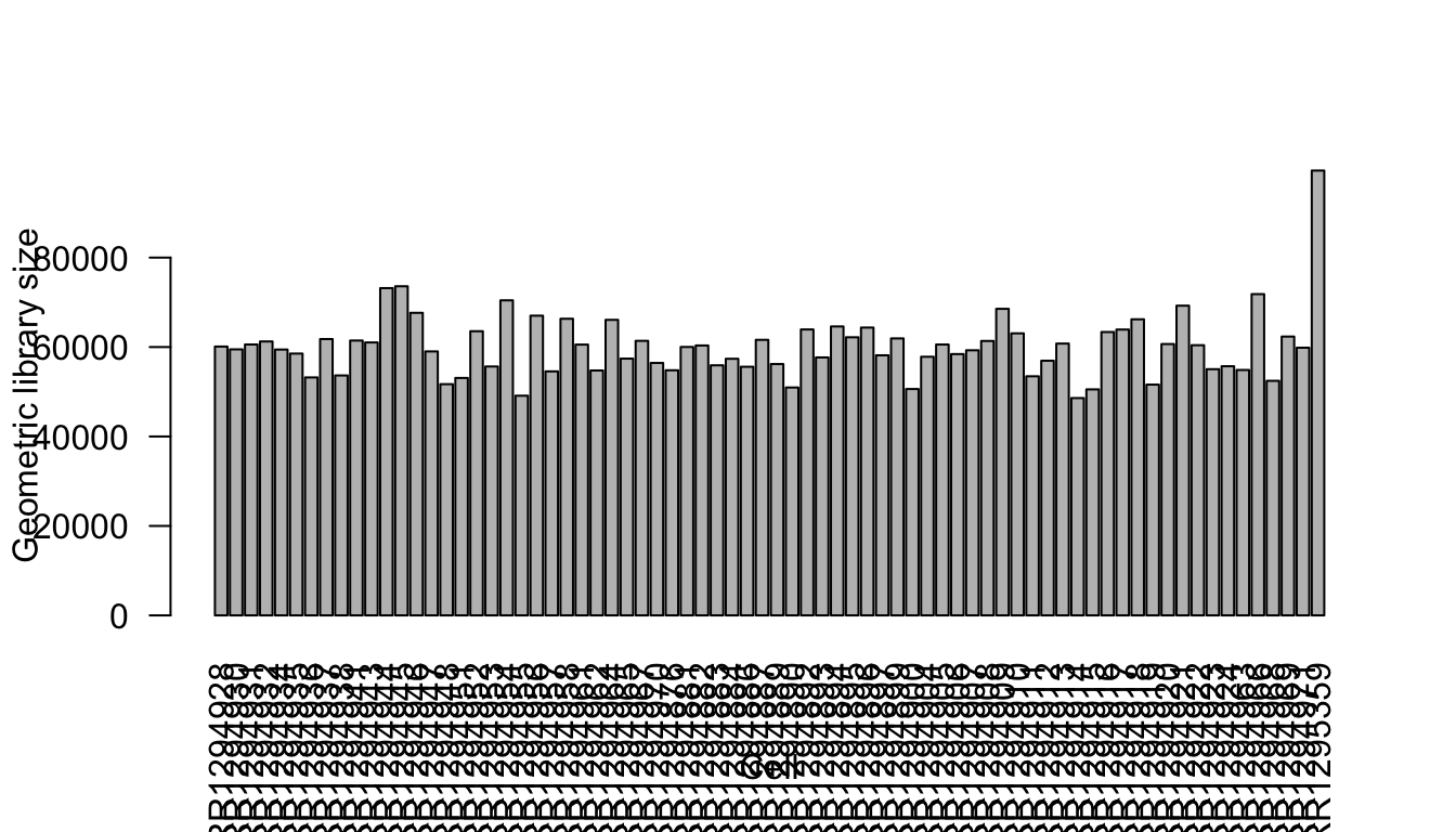

lcounts <- log(counts + 1)
# PC1 and Geometric library size correlation
pc1 = irlba(lcounts - rowMeans(lcounts), 1)$v[,1] ## partial SVD
cor(Num_Detected_Genes, pc1)

[1] 0.8357149

cor(Geo_Lib, pc1)

[1] 0.9299861

Run IA-SVA

Here, we run IA-SVA using Geo_Lib_Size as a known factor and identify five hidden factors. SVs are plotted in a pairwise fashion to uncover which SVs can seperate cells.

set.seed(3445)
mod <- model.matrix(~Geo_Lib)
summ_exp <- SummarizedExperiment(assays = counts)
iasva.res<- iasva(summ_exp, as.matrix(mod[,-1]),verbose=FALSE, permute=FALSE, num.sv=5)

IA-SVA running...


SV 1 Detected!


SV 2 Detected!


SV 3 Detected!


SV 4 Detected!


SV 5 Detected!


# of significant surrogate variables: 5

iasva.sv <- iasva.res$sv

Cluster <- as.factor(iasva.sv[,1] < 0.1) 
levels(Cluster)=c("Cluster1","Cluster2")
table(Cluster)

Cluster
Cluster1 Cluster2 
      13       61

pairs(iasva.sv[,1:5], main="IA-SVA", pch=21, col=color.vec[Cluster],
      bg=color.vec[Cluster], oma=c(4,4,6,14))
legend("right", levels(Cluster), fill=color.vec, bty="n")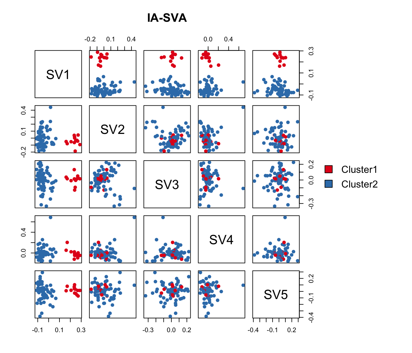

plot(iasva.sv[,1:2], main="IA-SVA", pch=21, xlab="SV1", ylab="SV2",
     col=color.vec[Cluster], bg=color.vec[Cluster])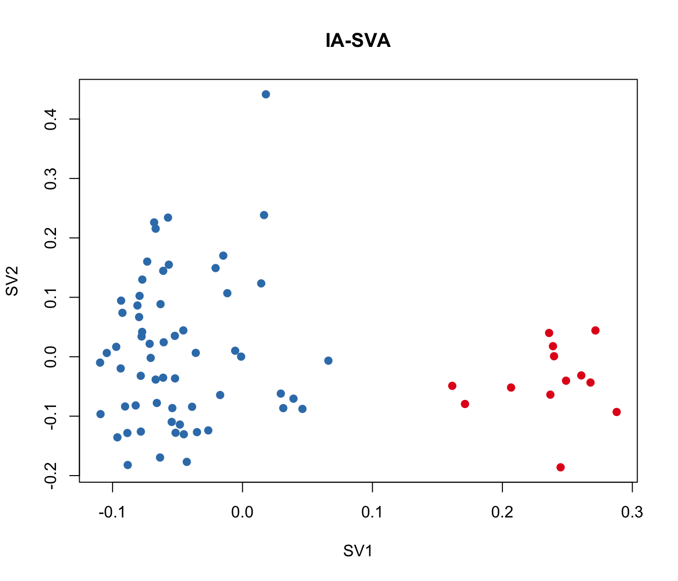

cor(Num_Detected_Genes, iasva.sv[,1])

[1] 0.3477167

cor(Geo_Lib, iasva.sv[,1])

[1] 0.4360903

corrplot(cor(iasva.sv))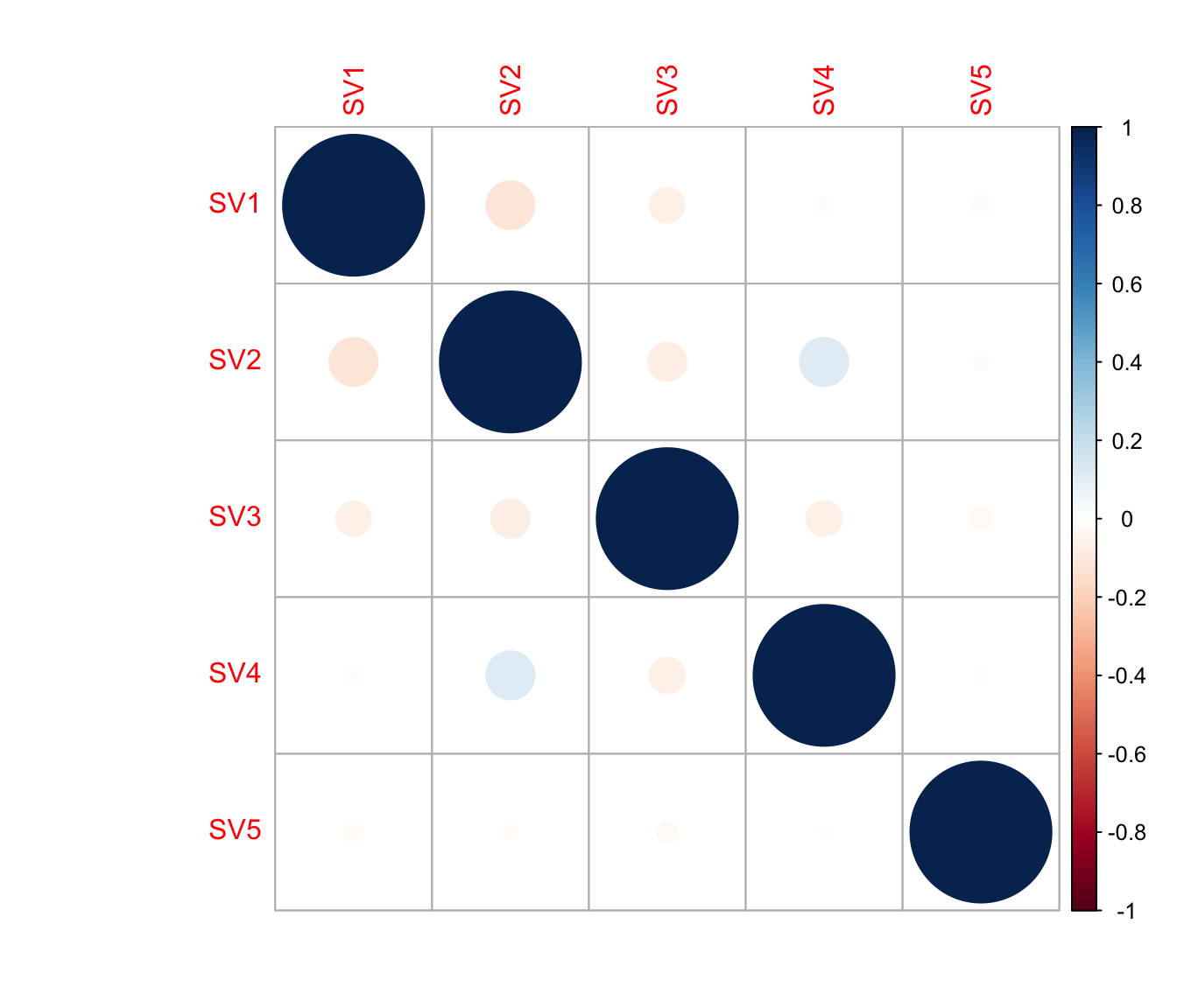

Find marker genes for the detected heterogeneity (SV1).

Here, using the find_markers() function we find marker genes that are significantly associated with SV1 (multiple testing adjusted p-value < 0.05, default significance cutoff, and R-squared value > 0.3).

# try different R2 thresholds
pdf(paste0("output/Clustering_analyses_figure3_sv1.pdf"))
r2.results <- study_R2(summ_exp, iasva.sv,selected.svs=1, no.clusters=2)

# of markers (): 466

total # of unique markers: 466

# of markers (): 361

total # of unique markers: 361

# of markers (): 232

total # of unique markers: 232

# of markers (): 165

total # of unique markers: 165

# of markers (): 119

total # of unique markers: 119

# of markers (): 89

total # of unique markers: 89

# of markers (): 62

total # of unique markers: 62

# of markers (): 47

total # of unique markers: 47

# of markers (): 33

total # of unique markers: 33

# of markers (): 21

total # of unique markers: 21

# of markers (): 14

total # of unique markers: 14

# of markers (): 5

total # of unique markers: 5

# of markers (): 1

total # of unique markers: 1

# of markers (): 0

total # of unique markers: 0

dev.off()

quartz_off_screen 
                2

marker.counts.SV1 <- find_markers(summ_exp, 
                            as.matrix(iasva.sv[,c(1)]), rsq.cutoff = 0.4)

# of markers (): 62

total # of unique markers: 62

marker.counts.SV1.long <- find_markers(summ_exp, 
                              as.matrix(iasva.sv[,c(1)]), rsq.cutoff = 0.3)

# of markers (): 119

total # of unique markers: 119

nrow(marker.counts.SV1)

[1] 62

nrow(marker.counts.SV1.long)

[1] 119

anno.col2 <- data.frame(Cluster=Cluster, SV1=iasva.sv[,1])
rownames(anno.col2) <- colnames(marker.counts.SV1)
head(anno.col2)

            Cluster         SV1
SRR1294928 Cluster2  0.03921618
SRR1294930 Cluster2 -0.08861064
SRR1294931 Cluster2 -0.06308121
SRR1294932 Cluster2 -0.07956245
SRR1294934 Cluster2  0.01656383
SRR1294935 Cluster2 -0.04288853

cluster.col <- color.vec[1:2]
names(cluster.col) <- as.vector(levels(Cluster))
anno.colors <- list(Cluster=cluster.col)
anno.colors

$Cluster
 Cluster1  Cluster2 
"#E41A1C" "#377EB8"

pheatmap(log(marker.counts.SV1+1), show_colnames =FALSE, 
         clustering_method = "ward.D2",cutree_cols = 2,annotation_col = anno.col2,
         annotation_colors = anno.colors)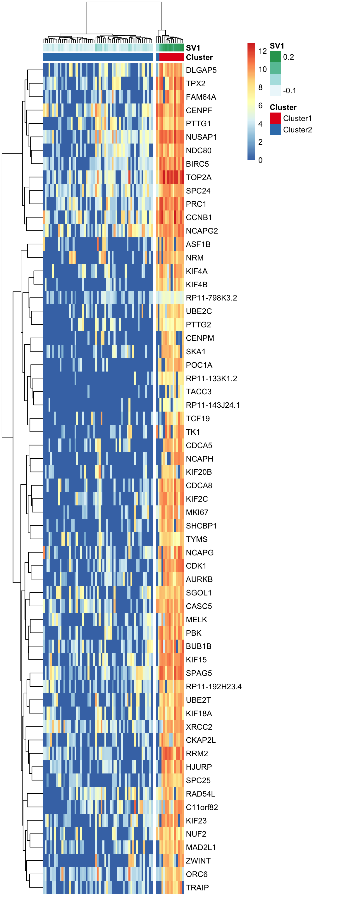

pheatmap(log(marker.counts.SV1.long+1), show_colnames =FALSE, 
         clustering_method = "ward.D2",cutree_cols = 2,annotation_col = anno.col2,
         annotation_colors = anno.colors)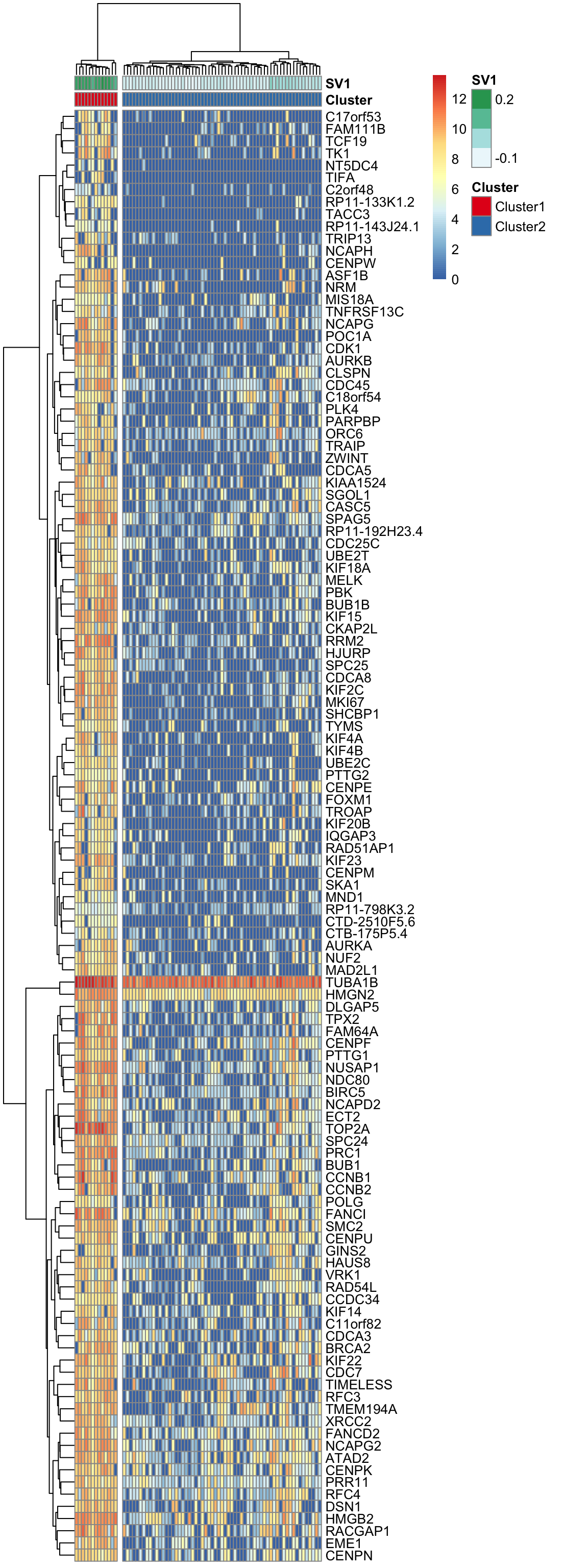

gene.list <- rownames(marker.counts.SV1)
write.table(gene.list, file = paste0("output/CC_genes.short.txt"),
            col.names =F, row.names = F, quote = F)

gene.list <- rownames(marker.counts.SV1.long)
write.table(gene.list, file = paste0("output/CC_genes.long.txt"),
            col.names =F, row.names = F, quote = F)

Theses marker genes are strongly enriched in cell-cycle related GO terms and KEGG pathways. (See Supplementary Figure 6 in https://doi.org/10.1101/151217)

Cell type assignment using scran R package

ENSG.counts <- counts
rownames(ENSG.counts) <- ENSG.ID
sce <- SingleCellExperiment(list(counts=ENSG.counts))

# load human cell cycle markers
hs.pairs <- readRDS(system.file("exdata", 
                                "human_cycle_markers.rds", package="scran"))
assigned <- cyclone(sce, pairs=hs.pairs)
head(assigned$scores)

     G1     S   G2M
1 0.432 0.983 0.001
2 0.103 0.926 0.027
3 0.105 0.895 0.009
4 0.032 0.950 0.024
5 0.003 0.692 0.560
6 0.452 0.905 0.000

table(assigned$phases)


 G1 G2M   S 
  8  14  52

phase <- rep("S", ncol(sce))
phase[assigned$scores$G1 > 0.5 & assigned$scores$G2M < 0.5] <- "G1"
phase[assigned$scores$G1 < 0.5 & assigned$scores$G2M > 0.5] <- "G2M"
phase[assigned$scores$G1 < 0.5 & assigned$scores$G2M < 0.5] <- "S"
phase[assigned$scores$G1 > 0.5 & assigned$scores$G2M > 0.5] <- "Unknown"
table(phase)

phase
     G1     G2M       S Unknown 
      7      12      52       3

G1 <- iasva.sv[,1][phase=="G1"]
S <- iasva.sv[,1][phase=="S"]
G2M <- iasva.sv[,1][phase=="G2M"]
Unknown <- iasva.sv[,1][phase=="Unknown"]
vioplot(G1, S, G2M, Unknown, names=c("G1", "S", "G2M", "Unknown"), 
   col="gold")
title(xlab="Cell-cycle stage predictions", ylab="IA-SVA factor (SV1)")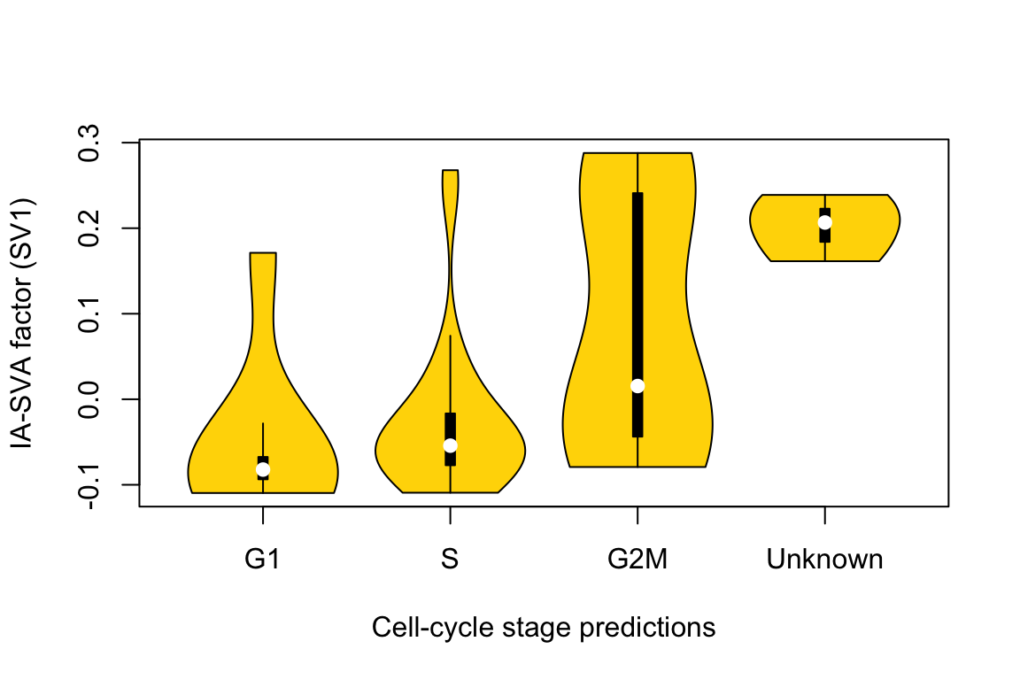

## Run tSNE to detect the hidden heterogeneity. For comparison purposes, we applied tSNE on read counts of all genes to identify the hidden heterogeneity. We used the Rtsne R package with default settings.

set.seed(43324)
tsne.res <- Rtsne(t(lcounts), dims = 2, perplexity = 20)
plot(tsne.res$Y, main="tSNE", xlab="Dim1", ylab="Dim2", 
     pch=21, col=color.vec[Cluster], bg=color.vec[Cluster], oma=c(4,4,6,12))
legend("bottomright", levels(Cluster), border="white",
       fill=color.vec, bty="n")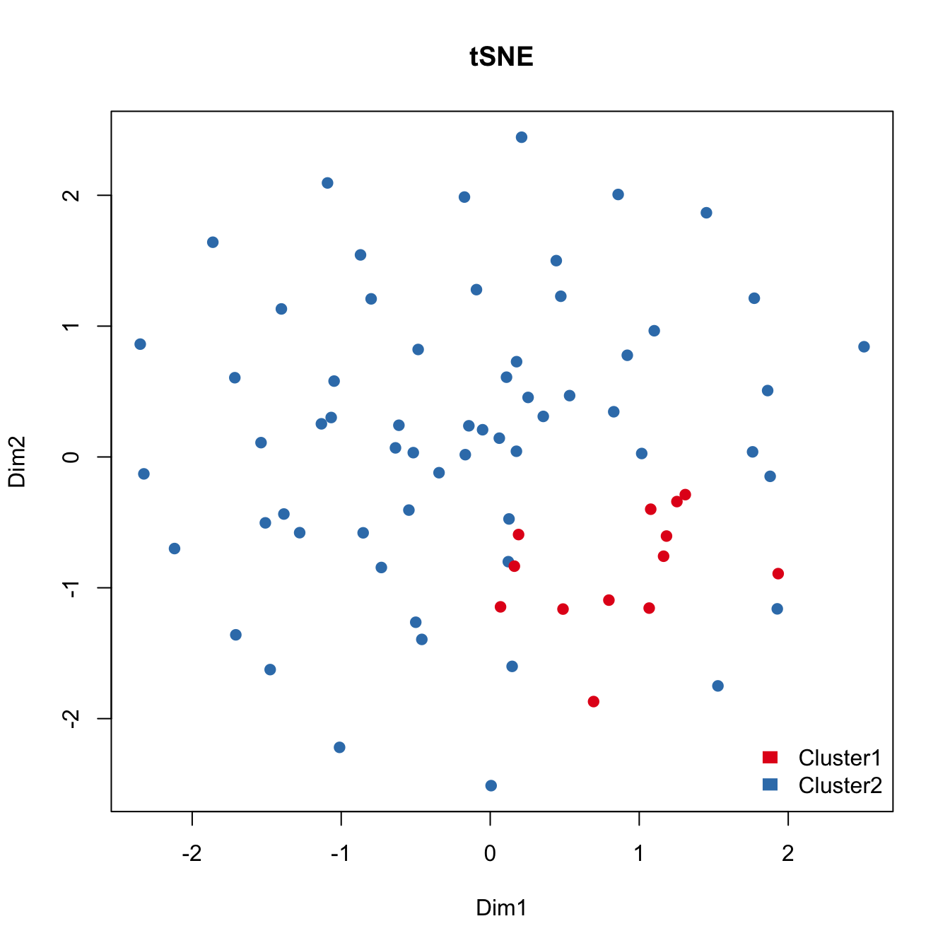

As shown above, tSNE fails to detect the outlier cells that are identified by IA-SVA when all genes are used. Same color coding is used as above.

Run tSNE post IA-SVA analyses, i.e., run tSNE on marker genes associated with SV1 as detected by IA-SVA.

Here, we apply tSNE on the marker genes for SV1 obtained from IA-SVA

set.seed(3452)
tsne.res <- Rtsne(unique(t(log(marker.counts.SV1.long+1))),
                  dims = 2, perplexity = 20)

plot(tsne.res$Y, main="IA-SVA + tSNE", xlab="tSNE Dim1",
     ylab="tSNE Dim2", pch=21, col=color.vec[Cluster],
     bg=color.vec[Cluster], oma=c(4,4,6,12))
legend("topright", levels(Cluster), border="white", fill=color.vec, bty="n")

Run principal component analysis (PCA) to detect the hidden heterogeneity (SV1).

Here, we use PCA to detect the cell cycle stage difference (SV1) detected by IA-SVA.

set.seed(3333)
pca.res = irlba(lcounts - rowMeans(lcounts), 5)$v ## partial SVD

pairs(pca.res[,1:5], main="PCA", pch=21, col=color.vec[Cluster],
      bg=color.vec[Cluster],
      oma=c(4,4,6,14))
legend("right", levels(Cluster), fill=color.vec, bty="n")

plot(pca.res[,1:2], main="PCA", pch=21, xlab="PC1", ylab="PC2",
     col=color.vec[Cluster], bg=color.vec[Cluster])
legend("bottomleft", levels(Cluster), border="white", fill=color.vec, bty="n")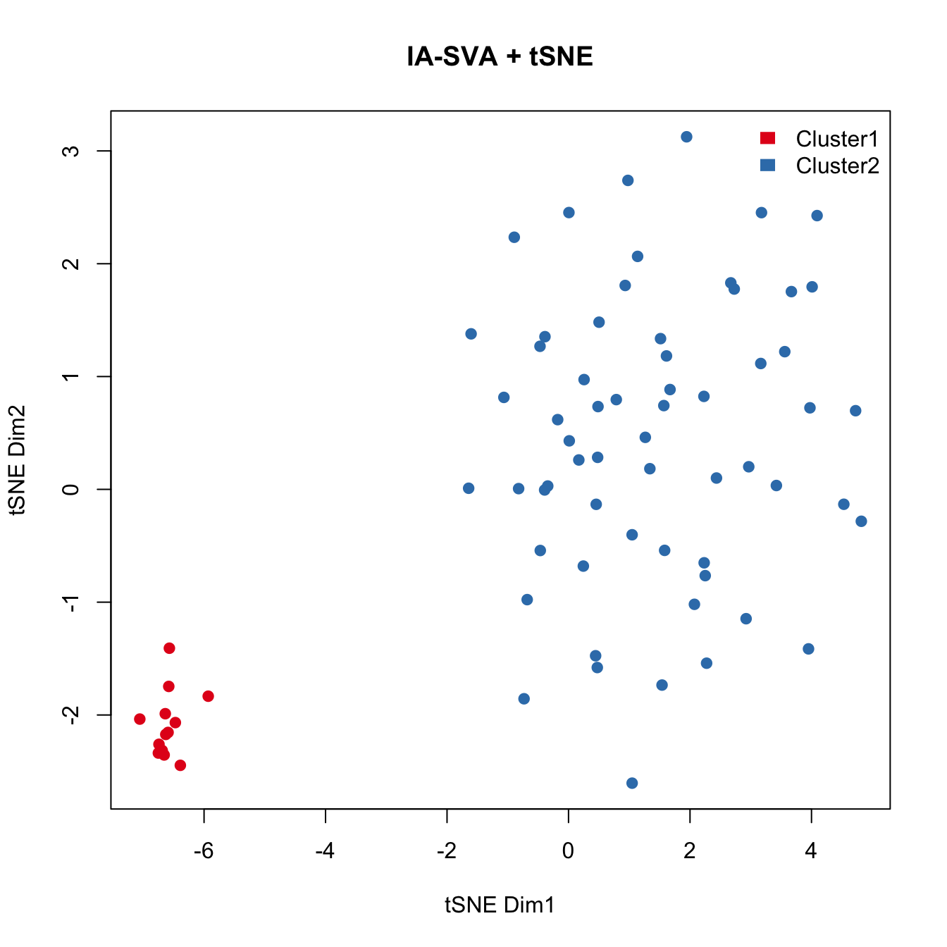

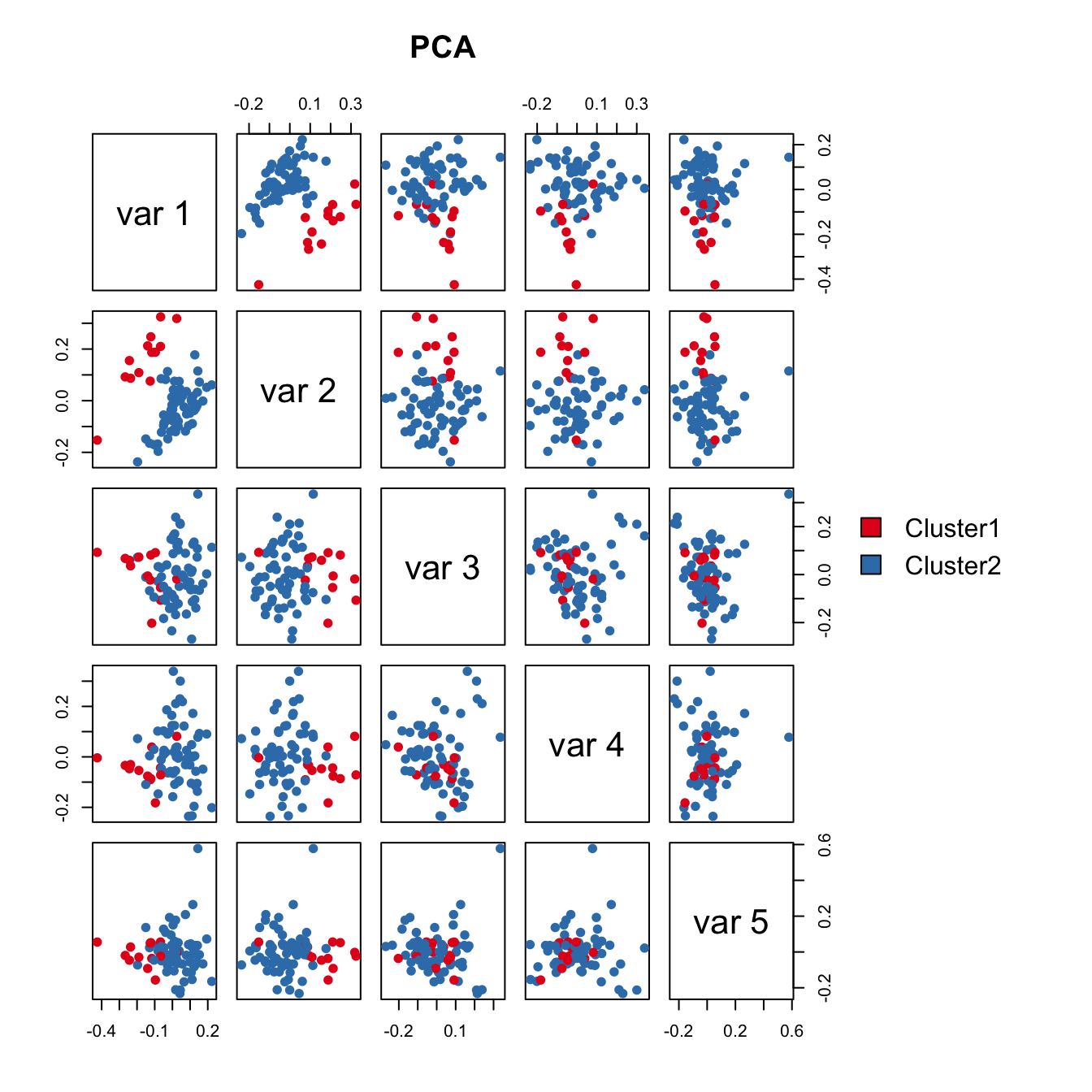
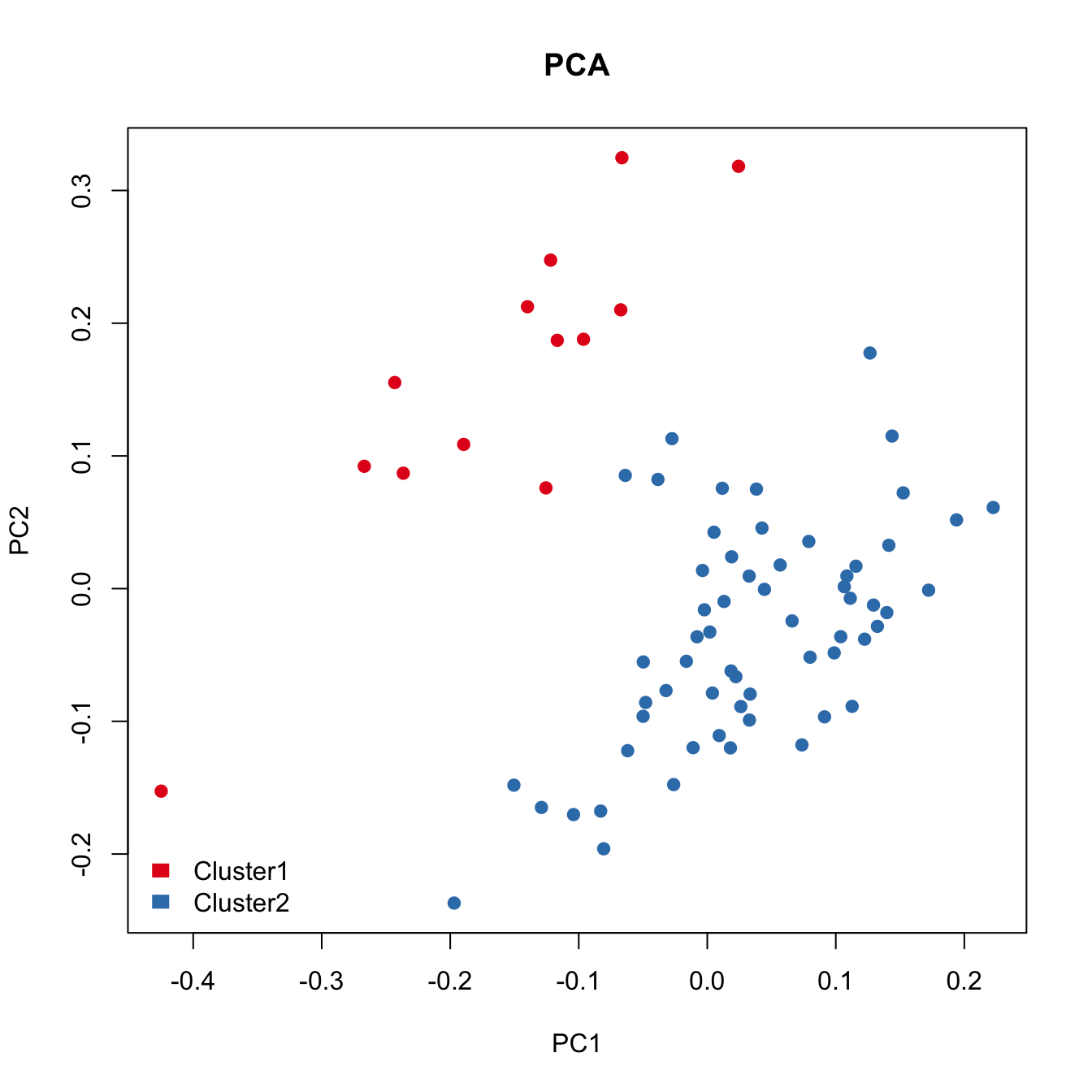PCA failed to capture the heterogeneity.

Run surrogate variable analysis (SVA) to detect the hidden heterogeneity (SV1).

Here, for comparison purposes we use SVA to detect the hidden heterogeneity in our example data.

mod1 <- model.matrix(~Geo_Lib)
mod0 <- cbind(mod1[,1])
sva.res = svaseq(counts,mod1,mod0, n.sv=5)$sv

Number of significant surrogate variables is:  5 
Iteration (out of 5 ):1  2  3  4  5

pairs(sva.res[,1:5], main="SVA", pch=21, col=color.vec[Cluster],
      bg=color.vec[Cluster], oma=c(4,4,6,14))
legend("right", levels(Cluster), border="white", fill=color.vec, bty="n")

plot(sva.res[,1:2], main="SVA", xlab="SV1", ylab="SV2",
     pch=21, col=color.vec[Cluster], bg=color.vec[Cluster])
legend("topleft", levels(Cluster), border="white", fill=color.vec, bty="n")

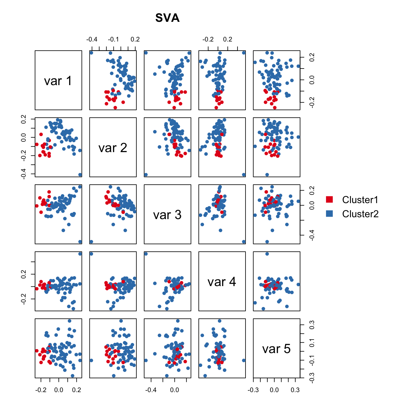
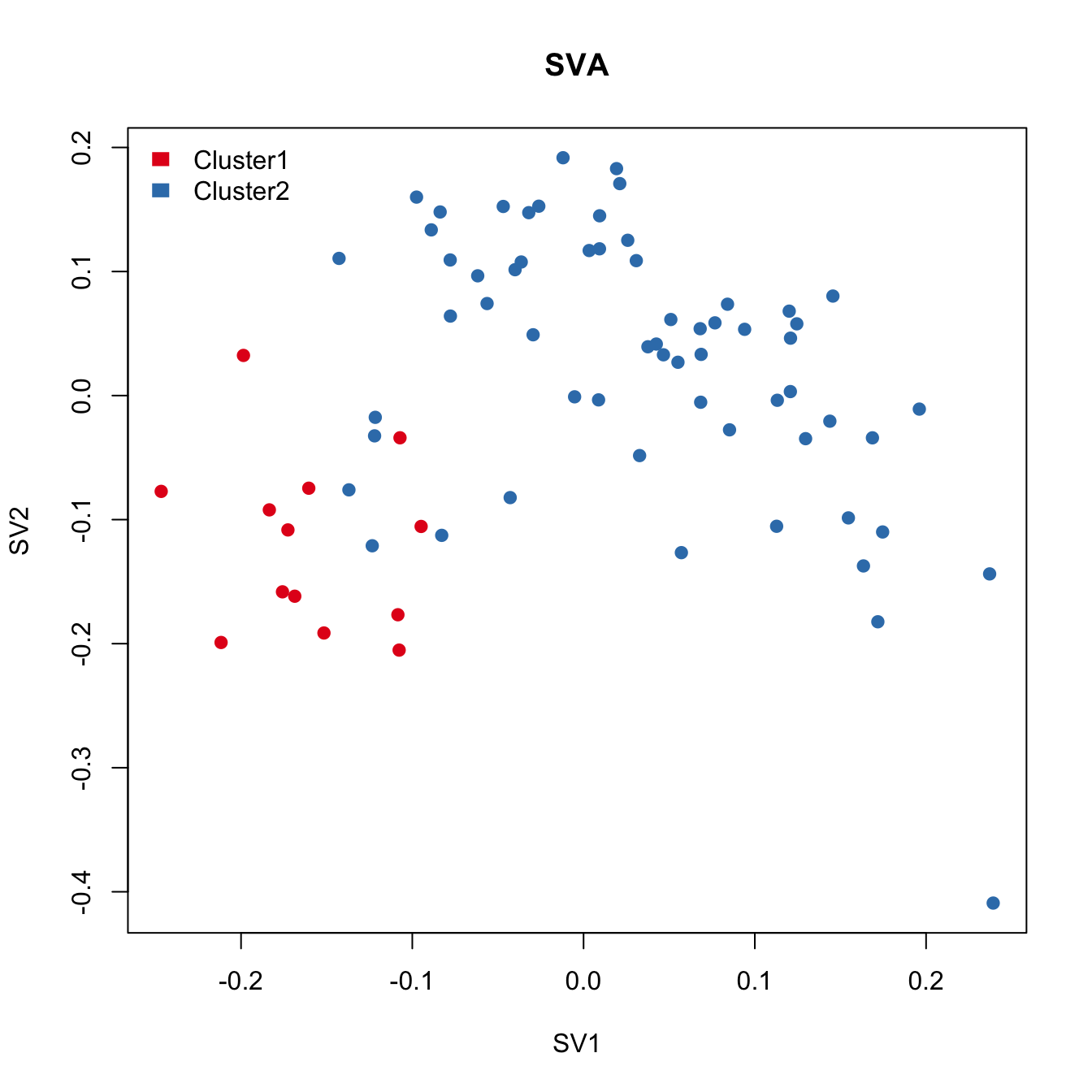SVA failed to detect the cell cycle stage difference.

Correlation between SV1 and the geometric library size

cor(Num_Detected_Genes, iasva.sv[,1])

[1] 0.3477167

cor(Geo_Lib, iasva.sv[,1])

[1] 0.4360903

By allowing correlation between factors, IA-SVA accurately detects the cell cycle stage difference, which is moderately correlated (|r|=0.44) with the geometric library size (the first principal component). Existing methods fail to detect the heterogeneity due to the orthogonality assumption.

pdf(file=paste0("output/Patel_Glioblastoma_MGH30_CellCycle_Figure3ABCD.pdf"), width=5, height=8)
layout(matrix(c(1,2,3,4,5,5), nrow=3, ncol=2, byrow=TRUE))
plot(iasva.sv[,1:2], main="IA-SVA", pch=21, xlab="SV1", ylab="SV2",
     col=color.vec[Cluster], bg=color.vec[Cluster], oma=c(4,4,6,12))
legend("topright", levels(Cluster), border="white", fill=color.vec, bty="n")
plot(pca.res[,1:2], main="PCA", pch=21, xlab="PC1", 
     ylab="PC2", col=color.vec[Cluster], bg=color.vec[Cluster])
plot(sva.res[,1:2], main="USVA", xlab="SV1", ylab="SV2",
     pch=21, col=color.vec[Cluster], bg=color.vec[Cluster])
plot(tsne.res$Y, main="tSNE", xlab="Dimension 1", 
     ylab="Dimension 2", pch=21, col=color.vec[Cluster], bg=color.vec[Cluster])
vioplot(G1, S, G2M, Unknown, names=c("G1", "S", "G2M", "Unknown"), 
   col="gold")
title(xlab="Cell-cycle stage predictions", ylab="IA-SVA factor")
dev.off()

quartz_off_screen 
                2

anno.col2 <- data.frame(Cluster=Cluster)
rownames(anno.col2) <- colnames(marker.counts.SV1)
head(anno.col2)

            Cluster
SRR1294928 Cluster2
SRR1294930 Cluster2
SRR1294931 Cluster2
SRR1294932 Cluster2
SRR1294934 Cluster2
SRR1294935 Cluster2

cluster.col <- color.vec[1:2]
names(cluster.col) <- as.vector(levels(Cluster))
anno.colors <- list(Cluster=cluster.col)
anno.colors

$Cluster
 Cluster1  Cluster2 
"#E41A1C" "#377EB8"

pheatmap(log(marker.counts.SV1.long+1), show_colnames =FALSE, 
         clustering_method = "ward.D2",cutree_cols = 2,annotation_col = anno.col2,
         annotation_colors = anno.colors)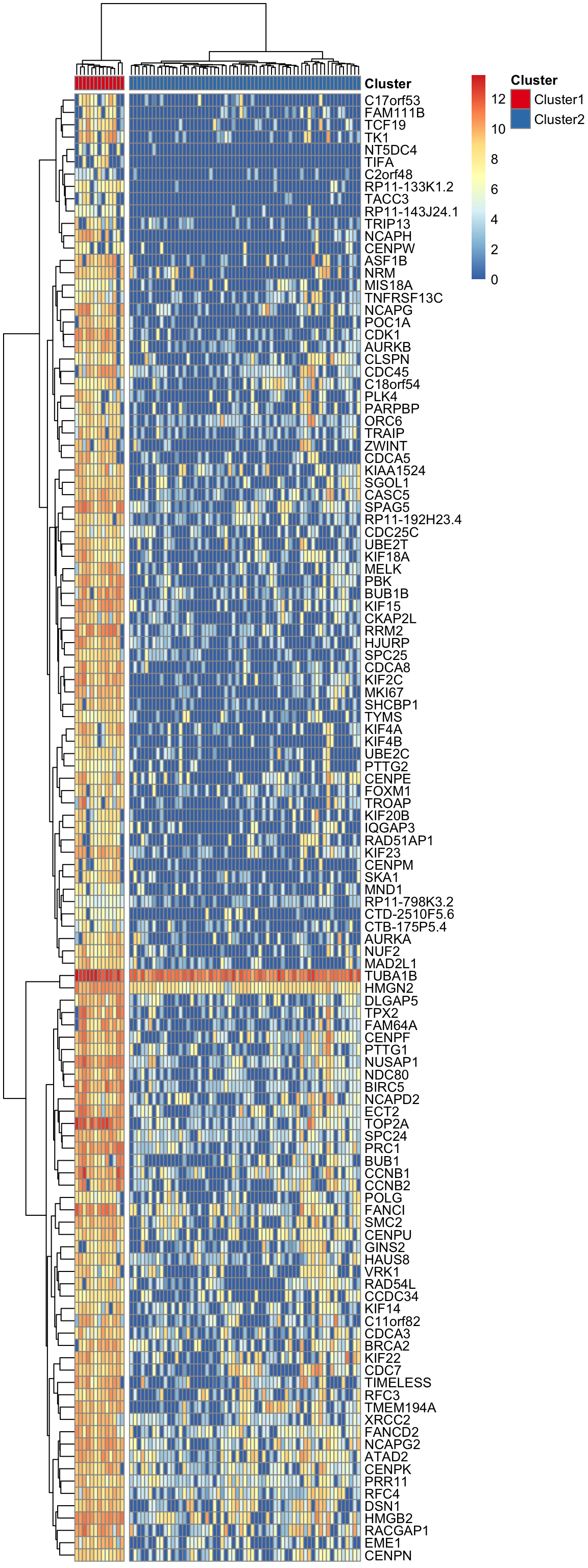

pheatmap(log(marker.counts.SV1.long+1), show_colnames =FALSE,
         clustering_method = "ward.D2",cutree_cols = 2,annotation_col = anno.col2,
         annotation_colors = anno.colors,
         filename=paste0("output/Patel_Glioblastoma_MGH30_iasva_SV1_genes_rsqcutoff0.3_pheatmap_iasvaV0.95_Figure3F.pdf"),
         width=6, height=16)

write.table(as.data.frame(rownames(marker.counts.SV1)), 
            file=paste0("output/Patel_Glioblastoma_MGH30_Cellcycle_SV1_Genes_rsqcutoff0.4.txt"),
            quote=F, row.names=F, col.names=F, sep=" ")

write.table(as.data.frame(rownames(marker.counts.SV1.long)), 
            file=paste0("output/Patel_Glioblastoma_MGH30_Cellcycle_SV1_Genes_rsqcutoff0.3.txt"), 
            quote=F, row.names=F, col.names=F, sep=" ")

Session information

sessionInfo()

R version 3.5.0 (2018-04-23)
Platform: x86_64-apple-darwin15.6.0 (64-bit)
Running under: macOS Sierra 10.12.6

Matrix products: default
BLAS: /Library/Frameworks/R.framework/Versions/3.5/Resources/lib/libRblas.0.dylib
LAPACK: /Library/Frameworks/R.framework/Versions/3.5/Resources/lib/libRlapack.dylib

locale:
[1] en_US.UTF-8/en_US.UTF-8/en_US.UTF-8/C/en_US.UTF-8/en_US.UTF-8

attached base packages:
[1] parallel  stats4    stats     graphics  grDevices utils     datasets 
[8] methods   base     

other attached packages:
 [1] vioplot_0.2                 sm_2.2-5.4                 
 [3] RColorBrewer_1.1-2          DescTools_0.99.24          
 [5] corrplot_0.84               pheatmap_1.0.10            
 [7] Rtsne_0.13                  scater_1.8.2               
 [9] ggplot2_2.2.1.9000          scran_1.8.2                
[11] SingleCellExperiment_1.2.0  SummarizedExperiment_1.10.1
[13] DelayedArray_0.6.1          matrixStats_0.53.1         
[15] Biobase_2.40.0              GenomicRanges_1.32.3       
[17] GenomeInfoDb_1.16.0         IRanges_2.14.10            
[19] S4Vectors_0.18.3            BiocGenerics_0.26.0        
[21] SCnorm_1.2.1                sva_3.28.0                 
[23] BiocParallel_1.14.2         genefilter_1.62.0          
[25] mgcv_1.8-23                 nlme_3.1-137               
[27] iasvaExamples_1.0.0         iasva_0.99.3               
[29] irlba_2.3.2                 Matrix_1.2-14              
[31] workflowr_1.0.1             rmarkdown_1.9              

loaded via a namespace (and not attached):
 [1] ggbeeswarm_0.6.0         colorspace_1.3-2        
 [3] rjson_0.2.19             dynamicTreeCut_1.63-1   
 [5] rprojroot_1.3-2          XVector_0.20.0          
 [7] MatrixModels_0.4-1       DT_0.4                  
 [9] bit64_0.9-7              manipulate_1.0.1        
[11] mvtnorm_1.0-8            AnnotationDbi_1.42.1    
[13] splines_3.5.0            R.methodsS3_1.7.1       
[15] tximport_1.8.0           knitr_1.20              
[17] annotate_1.58.0          cluster_2.0.7-1         
[19] R.oo_1.22.0              shinydashboard_0.7.0    
[21] shiny_1.1.0              compiler_3.5.0          
[23] backports_1.1.2          assertthat_0.2.0        
[25] lazyeval_0.2.1           limma_3.36.2            
[27] later_0.7.2              htmltools_0.3.6         
[29] quantreg_5.36            tools_3.5.0             
[31] bindrcpp_0.2.2           igraph_1.2.1            
[33] gtable_0.2.0             glue_1.2.0              
[35] GenomeInfoDbData_1.1.0   reshape2_1.4.3          
[37] dplyr_0.7.5              Rcpp_0.12.17            
[39] DelayedMatrixStats_1.2.0 stringr_1.3.1           
[41] mime_0.5                 statmod_1.4.30          
[43] XML_3.98-1.11            edgeR_3.22.3            
[45] MASS_7.3-50              zlibbioc_1.26.0         
[47] scales_0.5.0             promises_1.0.1          
[49] expm_0.999-2             rhdf5_2.24.0            
[51] SparseM_1.77             yaml_2.1.19             
[53] memoise_1.1.0            gridExtra_2.3           
[55] stringi_1.2.2            RSQLite_2.1.1           
[57] boot_1.3-20              rlang_0.2.1             
[59] pkgconfig_2.0.1          moments_0.14            
[61] bitops_1.0-6             evaluate_0.10.1         
[63] lattice_0.20-35          purrr_0.2.5             
[65] Rhdf5lib_1.2.1           bindr_0.1.1             
[67] labeling_0.3             htmlwidgets_1.2         
[69] bit_1.1-14               tidyselect_0.2.4        
[71] plyr_1.8.4               magrittr_1.5            
[73] R6_2.2.2                 DBI_1.0.0               
[75] foreign_0.8-70           pillar_1.2.3            
[77] whisker_0.3-2            withr_2.1.2             
[79] survival_2.42-3          RCurl_1.95-4.10         
[81] tibble_1.4.2             viridis_0.5.1           
[83] locfit_1.5-9.1           grid_3.5.0              
[85] data.table_1.11.4        blob_1.1.1              
[87] FNN_1.1                  git2r_0.21.0            
[89] digest_0.6.15            xtable_1.8-2            
[91] httpuv_1.4.3             R.utils_2.6.0           
[93] munsell_0.4.3            beeswarm_0.2.3          
[95] viridisLite_0.3.0        vipor_0.4.5

This reproducible R Markdown analysis was created with workflowr 1.0.1