Accuracy of SVs detected when hidden and known factors affect the overlapping sets of genes
Donghyung Lee
2018-08-01
- Install packages
- Load packages
- Load the islet single cell RNA-Seq data
- Look at mean variance relationship
- Estimate zero inflated negative binomial parameters from the islet data
- Generate a data set affected by two factors (known and unknown).
- Estimate hidden factor using IA-SVA
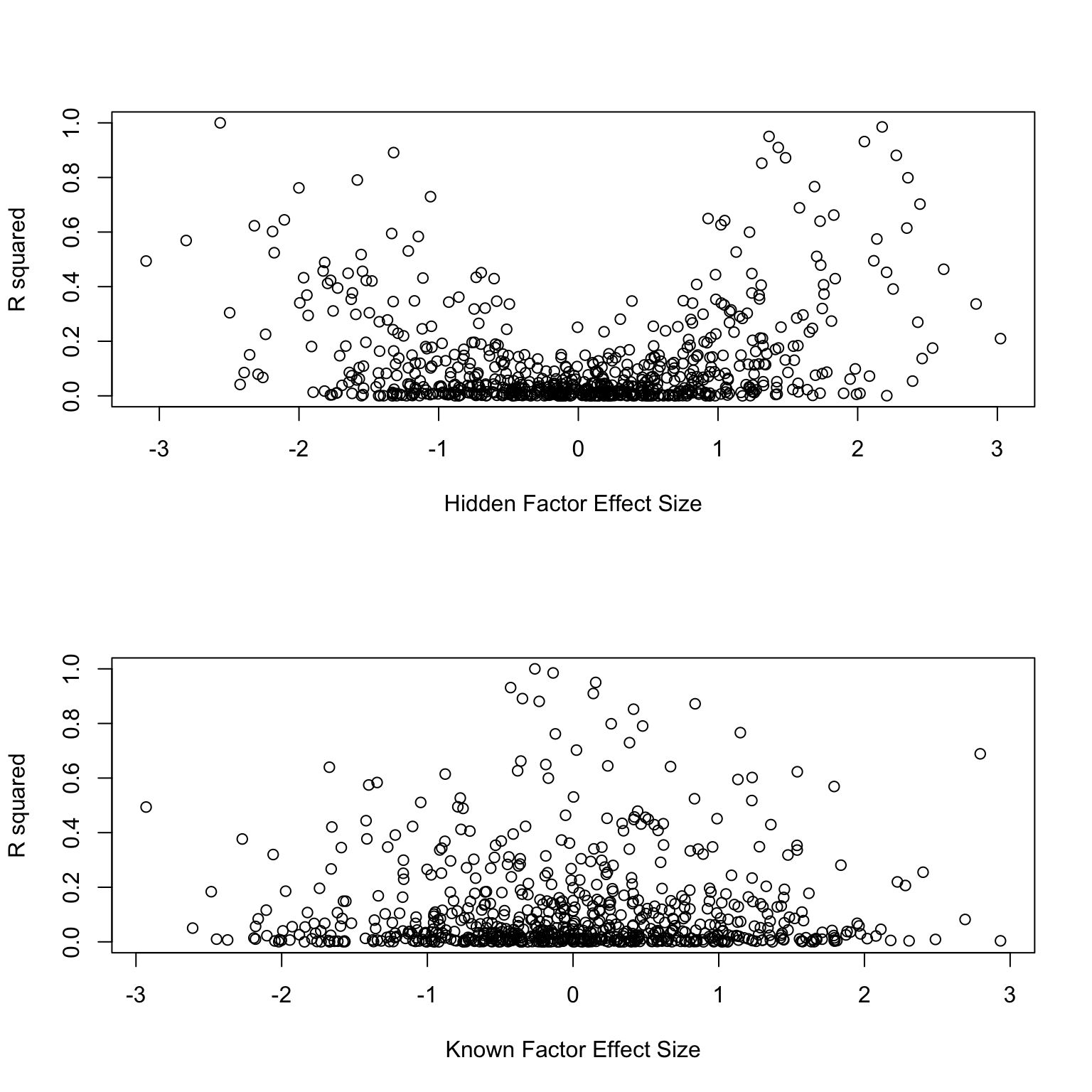
- R-squared (Weights) as a function of hidden and known factors’ effect size
- Hidden factor estimation using existing methods
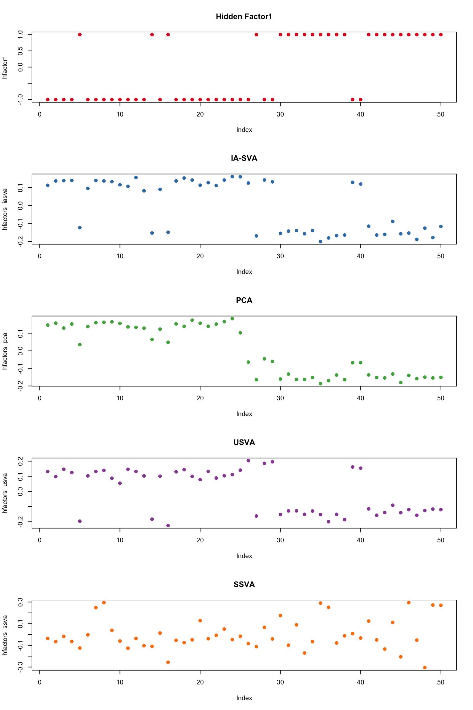
- Plot hidden factor estimates of IA-SVA and existing methods
- Multiple simulations where hidden and known factors affect overlapping sets of genes
- Estimation of hidden factors using IA-SVA and existing methods
- Compare the accuracy
- Session information
Last updated: 2018-08-01
workflowr checks: (Click a bullet for more information)-
✔ R Markdown file: up-to-date
Great! Since the R Markdown file has been committed to the Git repository, you know the exact version of the code that produced these results.
-
✔ Environment: empty
Great job! The global environment was empty. Objects defined in the global environment can affect the analysis in your R Markdown file in unknown ways. For reproduciblity it’s best to always run the code in an empty environment.
-
✔ Seed:
set.seed(20180731)The command
set.seed(20180731)was run prior to running the code in the R Markdown file. Setting a seed ensures that any results that rely on randomness, e.g. subsampling or permutations, are reproducible. -
✔ Session information: recorded
Great job! Recording the operating system, R version, and package versions is critical for reproducibility.
-
Great! You are using Git for version control. Tracking code development and connecting the code version to the results is critical for reproducibility. The version displayed above was the version of the Git repository at the time these results were generated.✔ Repository version: 5a96a44
Note that you need to be careful to ensure that all relevant files for the analysis have been committed to Git prior to generating the results (you can usewflow_publishorwflow_git_commit). workflowr only checks the R Markdown file, but you know if there are other scripts or data files that it depends on. Below is the status of the Git repository when the results were generated:
Note that any generated files, e.g. HTML, png, CSS, etc., are not included in this status report because it is ok for generated content to have uncommitted changes.Ignored files: Ignored: .DS_Store Ignored: .Rhistory Ignored: .Rproj.user/ Ignored: data/.DS_Store Ignored: inst/.DS_Store Ignored: inst/doc/.DS_Store Ignored: vignettes/.DS_Store Untracked files: Untracked: analysis/Brain_scRNASeq_neuron_vs_oligodendrocyte_single_run.Rmd Untracked: analysis/detecting_hidden_heterogeneity.Rmd Untracked: analysis/hidden_heterogeneity_glioblastoma.Rmd Untracked: analysis/reviewer2_sim.Rmd Untracked: analysis/scRNASeq_simulation.Rmd Untracked: analysis/tSNE_post_IA-SVA_3celltypes.Rmd Untracked: analysis/tSNE_post_IA-SVA_Xin_Islets.Rmd Untracked: docs/figure/ Untracked: output/GeneOverlap.Fig1.pdf Untracked: output/GeneOverlap.Fig2.pdf Untracked: output/absCor_gene_overlap_pct.pdf Untracked: output/gene_overlap.pdf Unstaged changes: Modified: analysis/_site.yml Deleted: analysis/about.Rmd Modified: analysis/index.Rmd Modified: analysis/license.Rmd
Expand here to see past versions:
Install packages
#devtools
library(devtools)
#iasva
devtools::install_github("UcarLab/IA-SVA")
#iasvaExamples
devtools::install_github("dleelab/iasvaExamples")
Load packages
rm(list=ls())
library(irlba) # partial SVD, the augmented implicitly restarted Lanczos bidiagonalization algorithm
library(iasva)
library(iasvaExamples)
library(sva)
library(polyester)
library(corrplot)
library(DescTools) #pcc i.e., Pearson's contingency coefficient
library(RColorBrewer)
library(reshape2)
library(ggplot2)
library(SummarizedExperiment)

color.vec <- brewer.pal(9, "Set1")

iasva.tmp <- function(Y, X, intercept=TRUE, num.sv=NULL, permute=TRUE, num.p=100, sig.cutoff= 0.05, threads=1, num.sv.permtest=NULL, tol=1e-10, verbose=FALSE){
  cat("IA-SVA running...")
  sv <- NULL
  pc.stat.obs <- NULL
  pval <- NULL
  wgt.mat <- NULL
  rsq <- NULL
  isv <- 0
  while(TRUE){
    if(!is.null(num.sv)){
      if(isv==num.sv){
        break
      }
    }
    iasva.res <- iasva.unit.tmp(Y, X, intercept, permute, num.p, threads, num.sv.permtest, tol, verbose)
    if(iasva.res$pval < sig.cutoff){
      sv <- cbind(sv, iasva.res$sv)
      pc.stat.obs <- cbind(pc.stat.obs, iasva.res$pc.stat.obs)
      pval <- c(pval, iasva.res$pval)
      wgt.mat <- cbind(wgt.mat, iasva.res$wgt)
      X <- cbind(X,iasva.res$sv)
    } else { break }
    isv <- isv+1
    cat(paste0("\nSV",isv, " Detected!"))
  }
  if (isv > 0) {
    colnames(sv) <- paste0("SV", 1:ncol(sv))
    cat(paste0("\n# of significant surrogate variables: ",length(pval)))
    return(list(sv=sv, pc.stat.obs=pc.stat.obs, pval=pval, n.sv=length(pval), wgt.mat=wgt.mat))
  } else {
    cat ("\nNo significant surrogate variables")
  }
}

iasva.unit.tmp <- function(Y, X, intercept=TRUE, permute=TRUE, num.p=100, threads=1, num.sv.permtest=NULL, tol=1e-10, verbose=FALSE){
  if(min(Y)<0){ Y <- Y + abs(min(Y)) }
  lY <- log(Y+1)
  if(intercept){
    fit <- .lm.fit(cbind(1,X), lY)
  } else {
    fit <- .lm.fit(X, lY)
  }
  resid <- resid(fit)
  tresid = t(resid)

  if(verbose) {cat("\n Perform SVD on residuals")}
  svd_pca <- irlba::irlba(tresid-rowMeans(tresid), 1, tol=tol)

  if(verbose) {cat("\n Regress residuals on PC1")}
  fit <- .lm.fit(cbind(1,svd_pca$v[,1]), resid)

  if(verbose) {cat("\n Get Rsq")}
  rsq.vec <- calc.rsq(resid, fit)

  if(verbose) {cat("\n Rsq 0-1 Normalization")}
  rsq.vec[is.na(rsq.vec)] <- min(rsq.vec, na.rm=TRUE)
  wgt <- (rsq.vec-min(rsq.vec))/(max(rsq.vec)-min(rsq.vec)) #0-1 normalization

  if(verbose) {cat("\n Obtain weighted log-transformed read counts")}
  tlY = t(lY)*wgt # weigh each row (gene) with respect to its Rsq value.

  if(verbose) {cat("\n Perform SVD on weighted log-transformed read counts")}
  sv <- irlba::irlba(tlY-rowMeans(tlY), 1, tol=tol)$v[,1]

  if(permute==TRUE){
    if(verbose) {cat("\n Assess the significance of the contribution of SV")}
    if(is.null(num.sv.permtest)){
      svd.res.obs <- svd(tresid - rowMeans(tresid))
    } else {
      svd.res.obs <- irlba::irlba(tresid-rowMeans(tresid), num.sv.permtest, tol=tol)
    }

    pc.stat.obs <- svd.res.obs$d[1]^2/sum(svd.res.obs$d^2)
    if(verbose) {cat("\n PC test statistic value:", pc.stat.obs)}

    # Generate an empirical null distribution of the PC test statistic.
    pc.stat.null.vec <- rep(0, num.p)
    permute.svd <- permute.svd.factory(lY, X, num.sv.permtest, tol, verbose)
    if (threads > 1) {
      threads <- min(threads, parallel::detectCores()-1)
      cl <- parallel::makeCluster(threads)
      pc.stat.null.vec <- tryCatch(parallel::parSapply(cl, 1:num.p, permute.svd), error=function(err){parallel::stopCluster(cl); stop(err)})
      parallel::stopCluster(cl)
    } else {
      pc.stat.null.vec <- sapply(1:num.p, permute.svd)
    }
    if(verbose) {cat("\n Empirical null distribution of the PC statistic:", sort(pc.stat.null.vec))}
    pval <- sum(pc.stat.obs <= pc.stat.null.vec)/(num.p+1)
    if(verbose) {cat("\n Permutation p-value:", pval)}
  } else {
    pc.stat.obs <- -1
    pval <- -1
  }
  return(list(sv=sv, pc.stat.obs=pc.stat.obs, pval=pval, wgt=wgt))
}

calc.rsq <- function(resid, fit) {
  RSS <- colSums(resid(fit)^2)
  TSS <- colSums(t(t(resid) - colSums(resid)/ncol(resid)) ^ 2)  # vectorized
  # TSS <- colSums(sweep(resid, 2, mean, "-") ^ 2)  # alt-2
  return(1-(RSS/(nrow(resid)-2))/(TSS/(nrow(resid)-1)))
}

permute.svd.factory <- function(lY, X, num.sv.permtest, tol, verbose) {

  permute.svd <- function(i) {
    permuted.lY <- apply(t(lY), 1, sample, replace=FALSE)
    tresid.null <- t(resid(.lm.fit(cbind(1,X), permuted.lY)))
    if(is.null(num.sv.permtest)) {
      svd.res.null <- svd(tresid.null)
    } else {
      svd.res.null <- irlba::irlba(tresid.null, num.sv.permtest, tol=tol)
    }
    return(svd.res.null$d[1]^2/sum(svd.res.null$d^2))
  }

  return(permute.svd)
}
Load the islet single cell RNA-Seq data
data("Lawlor_Islet_scRNAseq_Read_Counts")
data("Lawlor_Islet_scRNAseq_Annotations")
ls()
[1] "calc.rsq" "color.vec"
[3] "iasva.tmp" "iasva.unit.tmp"
[5] "Lawlor_Islet_scRNAseq_Annotations" "Lawlor_Islet_scRNAseq_Read_Counts"
[7] "permute.svd.factory" counts <- Lawlor_Islet_scRNAseq_Read_Counts
anns <- Lawlor_Islet_scRNAseq_Annotations
dim(anns)[1] 638 26dim(counts)[1] 26542 638summary(anns) run cell.type COL1A1 INS
Length:638 Length:638 Min. :1.00 Min. :1.000
Class :character Class :character 1st Qu.:1.00 1st Qu.:1.000
Mode :character Mode :character Median :1.00 Median :1.000
Mean :1.03 Mean :1.414
3rd Qu.:1.00 3rd Qu.:2.000
Max. :2.00 Max. :2.000
PRSS1 SST GCG KRT19
Min. :1.000 Min. :1.000 Min. :1.000 Min. :1.000
1st Qu.:1.000 1st Qu.:1.000 1st Qu.:1.000 1st Qu.:1.000
Median :1.000 Median :1.000 Median :1.000 Median :1.000
Mean :1.038 Mean :1.039 Mean :1.375 Mean :1.044
3rd Qu.:1.000 3rd Qu.:1.000 3rd Qu.:2.000 3rd Qu.:1.000
Max. :2.000 Max. :2.000 Max. :2.000 Max. :2.000
PPY num.genes Cell_ID UNOS_ID
Min. :1.000 Min. :3529 10th_C1_S59 : 1 ACCG268 :136
1st Qu.:1.000 1st Qu.:5270 10th_C10_S104: 1 ACJV399 :108
Median :1.000 Median :6009 10th_C11_S96 : 1 ACEL337 :103
Mean :1.028 Mean :5981 10th_C13_S61 : 1 ACIW009 : 93
3rd Qu.:1.000 3rd Qu.:6676 10th_C14_S53 : 1 ACCR015A: 57
Max. :2.000 Max. :8451 10th_C16_S105: 1 ACIB065 : 57
(Other) :632 (Other) : 84
Age Biomaterial_Provider Gender Phenotype
Min. :22.00 IIDP : 45 Female:303 Non-Diabetic :380
1st Qu.:29.00 Prodo Labs:593 Male :335 Type 2 Diabetic:258
Median :42.00
Mean :39.63
3rd Qu.:53.00
Max. :56.00
Race BMI Cell_Type Patient_ID
African American:175 Min. :22.00 INS :264 P1 :136
Hispanic :165 1st Qu.:26.60 GCG :239 P8 :108
White :298 Median :32.95 KRT19 : 28 P3 :103
Mean :32.85 SST : 25 P7 : 93
3rd Qu.:35.80 PRSS1 : 24 P5 : 57
Max. :55.00 none : 21 P6 : 57
(Other): 37 (Other): 84
Sequencing_Run Batch Coverage Percent_Aligned
12t : 57 B1:193 Min. :1206135 Min. :0.8416
4th : 57 B2:148 1st Qu.:2431604 1st Qu.:0.8769
9th : 57 B3:297 Median :3042800 Median :0.8898
10t : 56 Mean :3160508 Mean :0.8933
7th : 55 3rd Qu.:3871697 3rd Qu.:0.9067
3rd : 53 Max. :5931638 Max. :0.9604
(Other):303
Mitochondrial_Fraction Num_Expressed_Genes
Min. :0.003873 Min. :3529
1st Qu.:0.050238 1st Qu.:5270
Median :0.091907 Median :6009
Mean :0.108467 Mean :5981
3rd Qu.:0.142791 3rd Qu.:6676
Max. :0.722345 Max. :8451
ContCoef(table(anns$Gender, anns$Cell_Type))[1] 0.225969ContCoef(table(anns$Phenotype, anns$Cell_Type))[1] 0.1145096ContCoef(table(anns$Race, anns$Cell_Type))[1] 0.3084146ContCoef(table(anns$Patient_ID, anns$Cell_Type))[1] 0.5232058ContCoef(table(anns$Batch, anns$Cell_Type))[1] 0.3295619Look at mean variance relationship
plot(rowMeans(log(counts+1)),rowVars(log(counts+1)),pch=19,col=color.vec[2])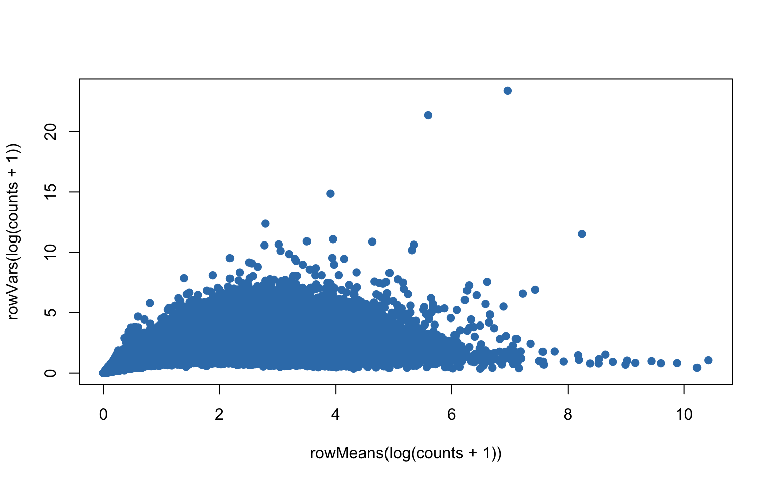
Estimate zero inflated negative binomial parameters from the islet data
## Estimate the zero inflated negative binomial parameters
params = get_params(counts)
Generate a data set affected by two factors (known and unknown).
Here we compare unsupervised SVA, supervised SVA and IA-SVA
set.seed(1234) #5000
sample.size <- 50
num.genes <- 10000
prop.kfactor.genes <- 0.2    #known factor
prop.hfactor1.genes <- 0.1   #hidden factor1

num.kfactor.genes <- num.genes*prop.kfactor.genes
num.hfactor1.genes <- num.genes*prop.hfactor1.genes

factor.prop <- 0.5
kfactor = c(rep(-1,each=sample.size*factor.prop),rep(1,each=sample.size-(sample.size*factor.prop)))
coinflip = rbinom(sample.size,size=1,prob=0.8)
hfactor1 = kfactor*coinflip + -kfactor*(1-coinflip)

cor(cbind(kfactor,hfactor1))
kfactor hfactor1
kfactor 1.0000000 0.6821865
hfactor1 0.6821865 1.0000000hfactor.mat <- cbind(hfactor1)
kfcoeffs = c(rnorm(num.kfactor.genes),rep(0,num.genes-num.kfactor.genes))
nullindex= (num.kfactor.genes+1):num.genes
overlap.prop <- 0.99
#hfcoeffs1 = c(rep(0,num.kfactor.genes*(1-overlap.prop)),rnorm(num.hfactor1.genes,sd=1),rep(0,num.genes-num.kfactor.genes*(1-overlap.prop)-num.hfactor1.genes))
hfcoeffs1 = c(rep(0,num.kfactor.genes-num.hfactor1.genes*overlap.prop),rnorm(num.hfactor1.genes,sd=1),rep(0,num.genes-(num.kfactor.genes-num.hfactor1.genes*overlap.prop)-num.hfactor1.genes))
par(mfrow=c(2,1))
plot(kfcoeffs)
plot(hfcoeffs1)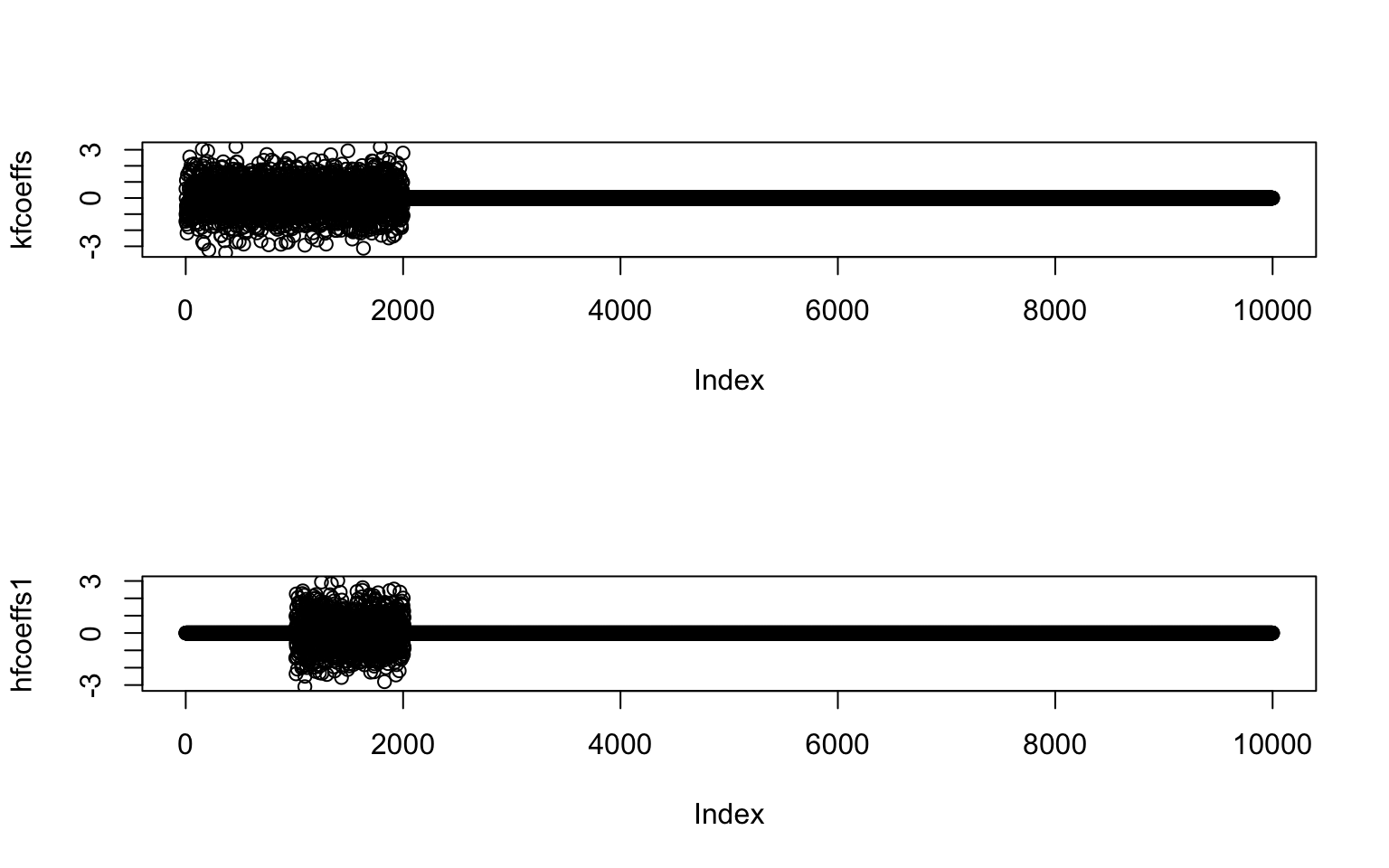
par(mfrow=c(1,1))

coeffs = cbind(hfcoeffs1,kfcoeffs)
controls = (hfcoeffs1!=0)&(kfcoeffs==0)
mod = model.matrix(~-1 + hfactor1 + kfactor)

dat0 = create_read_numbers(params$mu,params$fit,
                                     params$p0,beta=coeffs,mod=mod)
sum(dat0==0)/length(dat0)
[1] 0.680858filter = apply(dat0, 1, function(x) length(x[x>5])>=2)
dat0 = dat0[filter,]
sum(dat0==0)/length(dat0)[1] 0.5555512controls <- controls[filter]
dim(dat0)[1] 7067 50dim(mod)[1] 50 2
Compare the accuracy
iasva.cor.vec <- as.vector(abs(cor(hfactor1, do.call(cbind, hfactors_iasva_list))))
pca.cor.vec <- as.vector(abs(cor(hfactor1, do.call(cbind, hfactors_pca_list))))
usva.cor.vec <- as.vector(abs(cor(hfactor1, do.call(cbind, hfactors_usva_list))))
ssva.cor.vec <- as.vector(abs(cor(hfactor1, do.call(cbind, hfactors_ssva_list))))

cor.df <- data.frame(overlap.pct = 100*overlap.prop.vec,
                     IASVA = iasva.cor.vec,
                     PCA = pca.cor.vec,
                     USVA = usva.cor.vec,
                     SSVA = ssva.cor.vec)

melt.cor.df <- melt(cor.df, id.var=c("overlap.pct"))

p <- ggplot(melt.cor.df, aes(x=overlap.pct, y=value, group=variable))
p <- p + geom_line(aes(col=variable), size=1)
p <- p + geom_point(aes(col=variable), size=3)
p <- p + xlab("Gene Set Overlap Percentage")
p <- p + ylab("Absolute Correlation Coefficient")
#p <- p + scale_color_manual(values=color.vec)
p <- p + scale_color_brewer(palette = "Spectral", name="Method")
p <- p + theme_bw()
p <- p + theme(panel.border = element_blank(), panel.grid.major = element_blank(),
               #panel.grid.minor = element_blank(),
               axis.line = element_line(colour = "black"))
p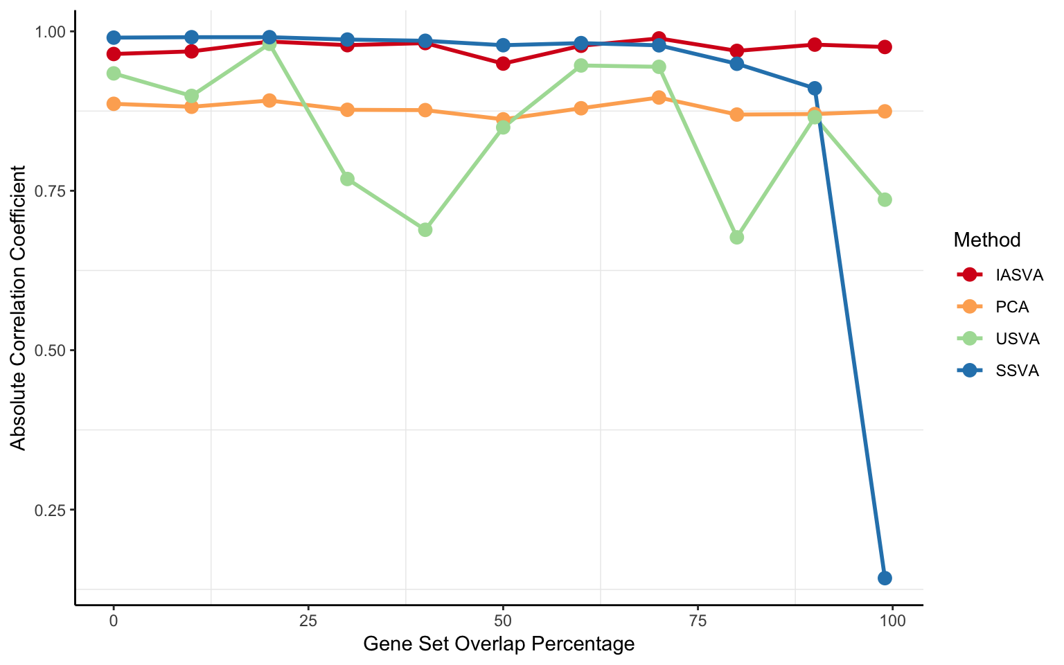
ggsave("output/absCor_gene_overlap_pct.pdf", width=8, height=5)Session information
sessionInfo()R version 3.5.0 (2018-04-23)
Platform: x86_64-apple-darwin15.6.0 (64-bit)
Running under: macOS Sierra 10.12.6
Matrix products: default
BLAS: /Library/Frameworks/R.framework/Versions/3.5/Resources/lib/libRblas.0.dylib
LAPACK: /Library/Frameworks/R.framework/Versions/3.5/Resources/lib/libRlapack.dylib
locale:
[1] en_US.UTF-8/en_US.UTF-8/en_US.UTF-8/C/en_US.UTF-8/en_US.UTF-8
attached base packages:
[1] parallel stats4 stats graphics grDevices utils datasets
[8] methods base
other attached packages:
[1] SummarizedExperiment_1.10.1 DelayedArray_0.6.1
[3] matrixStats_0.53.1 Biobase_2.40.0
[5] GenomicRanges_1.32.3 GenomeInfoDb_1.16.0
[7] IRanges_2.14.10 S4Vectors_0.18.3
[9] BiocGenerics_0.26.0 ggplot2_2.2.1.9000
[11] reshape2_1.4.3 RColorBrewer_1.1-2
[13] DescTools_0.99.24 corrplot_0.84
[15] polyester_1.16.0 sva_3.28.0
[17] BiocParallel_1.14.2 genefilter_1.62.0
[19] mgcv_1.8-23 nlme_3.1-137
[21] iasvaExamples_1.0.0 iasva_0.99.3
[23] irlba_2.3.2 Matrix_1.2-14
loaded via a namespace (and not attached):
[1] bitops_1.0-6 bit64_0.9-7 rprojroot_1.3-2
[4] tools_3.5.0 backports_1.1.2 R6_2.2.2
[7] DBI_1.0.0 lazyeval_0.2.1 colorspace_1.3-2
[10] withr_2.1.2 tidyselect_0.2.4 bit_1.1-14
[13] compiler_3.5.0 git2r_0.21.0 expm_0.999-2
[16] labeling_0.3 scales_0.5.0 mvtnorm_1.0-8
[19] stringr_1.3.1 digest_0.6.15 foreign_0.8-70
[22] rmarkdown_1.9 R.utils_2.6.0 XVector_0.20.0
[25] pkgconfig_2.0.1 htmltools_0.3.6 manipulate_1.0.1
[28] limma_3.36.2 rlang_0.2.1 RSQLite_2.1.1
[31] bindr_0.1.1 dplyr_0.7.5 R.oo_1.22.0
[34] RCurl_1.95-4.10 magrittr_1.5 GenomeInfoDbData_1.1.0
[37] Rcpp_0.12.17 munsell_0.4.3 R.methodsS3_1.7.1
[40] stringi_1.2.2 whisker_0.3-2 logspline_2.1.11
[43] yaml_2.1.19 MASS_7.3-50 zlibbioc_1.26.0
[46] plyr_1.8.4 grid_3.5.0 blob_1.1.1
[49] lattice_0.20-35 Biostrings_2.48.0 splines_3.5.0
[52] annotate_1.58.0 knitr_1.20 pillar_1.2.3
[55] boot_1.3-20 XML_3.98-1.11 glue_1.2.0
[58] evaluate_0.10.1 gtable_0.2.0 purrr_0.2.5
[61] assertthat_0.2.0 xtable_1.8-2 survival_2.42-3
[64] tibble_1.4.2 AnnotationDbi_1.42.1 memoise_1.1.0
[67] workflowr_1.0.1 bindrcpp_0.2.2 cluster_2.0.7-1 This reproducible R Markdown analysis was created with workflowr 1.0.1