IA-SVA based feature selection improves the performance of clustering algorithms [1]

Load packages
Load the islet single cell RNA-Seq data
Extract three cell types (GCG (alpha), INS (beta), KRT19 (ductal) expressing cells) from healthy (i.e., non-diabetic) subjects and filter out low-expressed genes
Calculate the number of detected genes
Run tSNE to cluster islet cells.
Run IA-SVA
Find marker genes for SV1 and SV3.
Find marker genes for SV4.
Run tSNE post IA-SVA, i.e., run tSNE on marker genes for SV1 and SV2 obtained from IA-SVA.
Run CellView algorithm to visualize the data.
Run Seurat to reduce dimensionality and visualize islet cells
Session information

Last updated: 2018-08-03

workflowr checks: (Click a bullet for more information)

✔ R Markdown file: up-to-date

Great! Since the R Markdown file has been committed to the Git repository, you know the exact version of the code that produced these results.
✔ Environment: empty

Great job! The global environment was empty. Objects defined in the global environment can affect the analysis in your R Markdown file in unknown ways. For reproduciblity it’s best to always run the code in an empty environment.
✔ Seed: set.seed(20180731)

The command set.seed(20180731) was run prior to running the code in the R Markdown file. Setting a seed ensures that any results that rely on randomness, e.g. subsampling or permutations, are reproducible.
✔ Session information: recorded

Great job! Recording the operating system, R version, and package versions is critical for reproducibility.
✔ Repository version: 2689835
Great! You are using Git for version control. Tracking code development and connecting the code version to the results is critical for reproducibility. The version displayed above was the version of the Git repository at the time these results were generated.

Note that you need to be careful to ensure that all relevant files for the analysis have been committed to Git prior to generating the results (you can use wflow_publish or wflow_git_commit). workflowr only checks the R Markdown file, but you know if there are other scripts or data files that it depends on. Below is the status of the Git repository when the results were generated:
```
Ignored files:
    Ignored:    .DS_Store
    Ignored:    .Rhistory
    Ignored:    .Rproj.user/
    Ignored:    data/.DS_Store
    Ignored:    inst/.DS_Store
    Ignored:    inst/doc/.DS_Store
    Ignored:    vignettes/.DS_Store

Untracked files:
    Untracked:  docs/figure/hidden_heterogeneity_glioblastoma.Rmd/
    Untracked:  output/CC_genes.long.txt
    Untracked:  output/CC_genes.short.txt
    Untracked:  output/Clustering_analyses_figure3_sv1.pdf
    Untracked:  output/Patel_Glioblastoma_MGH30_CellCycle_Figure3ABCD.pdf
    Untracked:  output/Patel_Glioblastoma_MGH30_Cellcycle_SV1_Genes_rsqcutoff0.3.txt
    Untracked:  output/Patel_Glioblastoma_MGH30_Cellcycle_SV1_Genes_rsqcutoff0.4.txt
    Untracked:  output/Patel_Glioblastoma_MGH30_iasva_SV1_genes_rsqcutoff0.3_pheatmap_iasvaV0.95_Figure3F.pdf
```
Note that any generated files, e.g. HTML, png, CSS, etc., are not included in this status report because it is ok for generated content to have uncommitted changes.

Expand here to see past versions:

File	Version	Author	Date	Message
Rmd	c241b04	dleelab	2018-08-03	added
html	c241b04	dleelab	2018-08-03	added

The IA-SVA based feature selection can significantly improve the performance and utility of clustering algorithms (e.g., tSNE, hierarchical clustering). To illustrate how the IA-SVA method can be used to improve the performance of clustering algorithms, we used real-world single cell RNA sequencing (scRNA-Seq) data obtained from human pancreatic islet samples (Lawlor et. al., 2016). This dataset is included in a R data package (“iasvaExamples”) containing data examples for IA-SVA (https://github.com/dleelab/iasvaExamples). To install the ‘iasvaExamples’ package, follow the instruction provided in the GitHub page.

Load packages

rm(list=ls())
library(irlba)

Loading required package: Matrix

library(iasva)
library(iasvaExamples)
library(Seurat)

Loading required package: ggplot2

Loading required package: cowplot


Attaching package: 'cowplot'

The following object is masked from 'package:ggplot2':

    ggsave

library(dbscan)
library(Rtsne)
library(pheatmap)
library(corrplot)

corrplot 0.84 loaded

library(DescTools) #pcc i.e., Pearson's contingency coefficient
library(RColorBrewer)
library(SummarizedExperiment)

Loading required package: GenomicRanges

Loading required package: stats4

Loading required package: BiocGenerics

Loading required package: parallel


Attaching package: 'BiocGenerics'

The following objects are masked from 'package:parallel':

    clusterApply, clusterApplyLB, clusterCall, clusterEvalQ,
    clusterExport, clusterMap, parApply, parCapply, parLapply,
    parLapplyLB, parRapply, parSapply, parSapplyLB

The following objects are masked from 'package:Matrix':

    colMeans, colSums, rowMeans, rowSums, which

The following objects are masked from 'package:stats':

    IQR, mad, sd, var, xtabs

The following objects are masked from 'package:base':

    anyDuplicated, append, as.data.frame, basename, cbind,
    colMeans, colnames, colSums, dirname, do.call, duplicated,
    eval, evalq, Filter, Find, get, grep, grepl, intersect,
    is.unsorted, lapply, lengths, Map, mapply, match, mget, order,
    paste, pmax, pmax.int, pmin, pmin.int, Position, rank, rbind,
    Reduce, rowMeans, rownames, rowSums, sapply, setdiff, sort,
    table, tapply, union, unique, unsplit, which, which.max,
    which.min

Loading required package: S4Vectors


Attaching package: 'S4Vectors'

The following object is masked from 'package:Matrix':

    expand

The following object is masked from 'package:base':

    expand.grid

Loading required package: IRanges

Loading required package: GenomeInfoDb

Loading required package: Biobase

Welcome to Bioconductor

    Vignettes contain introductory material; view with
    'browseVignettes()'. To cite Bioconductor, see
    'citation("Biobase")', and for packages 'citation("pkgname")'.

Loading required package: DelayedArray

Loading required package: matrixStats


Attaching package: 'matrixStats'

The following objects are masked from 'package:Biobase':

    anyMissing, rowMedians

Loading required package: BiocParallel


Attaching package: 'DelayedArray'

The following objects are masked from 'package:matrixStats':

    colMaxs, colMins, colRanges, rowMaxs, rowMins, rowRanges

The following objects are masked from 'package:base':

    aperm, apply

color.vec <- brewer.pal(8, "Set1")
# Normalization.
normalize <- function (counts) 
{
    normfactor <- colSums(counts)
    return(t(t(counts)/normfactor)*median(normfactor))
}

Load the islet single cell RNA-Seq data

data("Lawlor_Islet_scRNAseq_Read_Counts")
data("Lawlor_Islet_scRNAseq_Annotations")
ls()

[1] "color.vec"                         "Lawlor_Islet_scRNAseq_Annotations"
[3] "Lawlor_Islet_scRNAseq_Read_Counts" "normalize"

counts <- Lawlor_Islet_scRNAseq_Read_Counts
anns <- Lawlor_Islet_scRNAseq_Annotations
dim(anns)

[1] 638  26

dim(counts)

[1] 26542   638

summary(anns)

     run             cell.type             COL1A1          INS       
 Length:638         Length:638         Min.   :1.00   Min.   :1.000  
 Class :character   Class :character   1st Qu.:1.00   1st Qu.:1.000  
 Mode  :character   Mode  :character   Median :1.00   Median :1.000  
                                       Mean   :1.03   Mean   :1.414  
                                       3rd Qu.:1.00   3rd Qu.:2.000  
                                       Max.   :2.00   Max.   :2.000  
                                                                     
     PRSS1            SST             GCG            KRT19      
 Min.   :1.000   Min.   :1.000   Min.   :1.000   Min.   :1.000  
 1st Qu.:1.000   1st Qu.:1.000   1st Qu.:1.000   1st Qu.:1.000  
 Median :1.000   Median :1.000   Median :1.000   Median :1.000  
 Mean   :1.038   Mean   :1.039   Mean   :1.375   Mean   :1.044  
 3rd Qu.:1.000   3rd Qu.:1.000   3rd Qu.:2.000   3rd Qu.:1.000  
 Max.   :2.000   Max.   :2.000   Max.   :2.000   Max.   :2.000  
                                                                
      PPY          num.genes             Cell_ID        UNOS_ID   
 Min.   :1.000   Min.   :3529   10th_C1_S59  :  1   ACCG268 :136  
 1st Qu.:1.000   1st Qu.:5270   10th_C10_S104:  1   ACJV399 :108  
 Median :1.000   Median :6009   10th_C11_S96 :  1   ACEL337 :103  
 Mean   :1.028   Mean   :5981   10th_C13_S61 :  1   ACIW009 : 93  
 3rd Qu.:1.000   3rd Qu.:6676   10th_C14_S53 :  1   ACCR015A: 57  
 Max.   :2.000   Max.   :8451   10th_C16_S105:  1   ACIB065 : 57  
                                (Other)      :632   (Other) : 84  
      Age        Biomaterial_Provider    Gender              Phenotype  
 Min.   :22.00   IIDP      : 45       Female:303   Non-Diabetic   :380  
 1st Qu.:29.00   Prodo Labs:593       Male  :335   Type 2 Diabetic:258  
 Median :42.00                                                          
 Mean   :39.63                                                          
 3rd Qu.:53.00                                                          
 Max.   :56.00                                                          
                                                                        
               Race          BMI          Cell_Type     Patient_ID 
 African American:175   Min.   :22.00   INS    :264   P1     :136  
 Hispanic        :165   1st Qu.:26.60   GCG    :239   P8     :108  
 White           :298   Median :32.95   KRT19  : 28   P3     :103  
                        Mean   :32.85   SST    : 25   P7     : 93  
                        3rd Qu.:35.80   PRSS1  : 24   P5     : 57  
                        Max.   :55.00   none   : 21   P6     : 57  
                                        (Other): 37   (Other): 84  
 Sequencing_Run Batch       Coverage       Percent_Aligned 
 12t    : 57    B1:193   Min.   :1206135   Min.   :0.8416  
 4th    : 57    B2:148   1st Qu.:2431604   1st Qu.:0.8769  
 9th    : 57    B3:297   Median :3042800   Median :0.8898  
 10t    : 56             Mean   :3160508   Mean   :0.8933  
 7th    : 55             3rd Qu.:3871697   3rd Qu.:0.9067  
 3rd    : 53             Max.   :5931638   Max.   :0.9604  
 (Other):303                                               
 Mitochondrial_Fraction Num_Expressed_Genes
 Min.   :0.003873       Min.   :3529       
 1st Qu.:0.050238       1st Qu.:5270       
 Median :0.091907       Median :6009       
 Mean   :0.108467       Mean   :5981       
 3rd Qu.:0.142791       3rd Qu.:6676       
 Max.   :0.722345       Max.   :8451

ContCoef(table(anns$Gender, anns$Cell_Type))

[1] 0.225969

ContCoef(table(anns$Phenotype, anns$Cell_Type))

[1] 0.1145096

ContCoef(table(anns$Race, anns$Cell_Type))

[1] 0.3084146

ContCoef(table(anns$Patient_ID, anns$Cell_Type))

[1] 0.5232058

ContCoef(table(anns$Batch, anns$Cell_Type))

[1] 0.3295619

The annotations describing the islet samples and experimental settings are stored in “anns” and the read counts information is stored in “counts”.

Extract three cell types (GCG (alpha), INS (beta), KRT19 (ductal) expressing cells) from healthy (i.e., non-diabetic) subjects and filter out low-expressed genes

counts <- counts[, (anns$Phenotype!="Non-Diabetic")&
                    ((anns$Cell_Type=="GCG")|
                      (anns$Cell_Type=="INS")|
                        (anns$Cell_Type=="KRT19"))]
anns <- subset(anns, (Phenotype!="Non-Diabetic")& 
                      ((Cell_Type=="GCG")|
                        (Cell_Type=="INS")|
                          (Cell_Type=="KRT19")))
dim(counts)

[1] 26542 213

dim(anns)

[1] 213 26

anns <- droplevels(anns)
prop.zeros <- sum(counts==0)/length(counts)
prop.zeros

[1] 0.6917875

filter = apply(counts, 1, function(x) length(x[x>5])>=3)
counts = counts[filter,]
dim(counts)

[1] 16005 213

prop.zeros <- sum(counts==0)/length(counts)
prop.zeros

[1] 0.4956072

Patient_ID <- anns$Patient_ID
Cell_Type <- anns$Cell_Type
levels(Cell_Type) <- c("alpha", "beta", "ductal")
Batch <- anns$Batch
table(Cell_Type)

Cell_Type alpha beta ductal 101 96 16

raw.counts <- counts
summary(colSums(counts))

Min. 1st Qu. Median Mean 3rd Qu. Max. 473182 1014530 1263975 1310323 1492478 3090459

counts <- normalize(counts)
summary(colSums(counts))

Min. 1st Qu. Median Mean 3rd Qu. Max. 1263975 1263975 1263975 1263975 1263975 1263975

Calculate the number of detected genes

It is well known that the number of detected genes in each cell explains a very large portion of variability in scRNA-Seq data (Hicks et. al. 2015 BioRxiv, McDavid et. al. 2016 Nature Biotechnology). Frequently, the first principal component of log-transformed scRNA-Seq read counts is highly correlated with the number of detected genes (e.g., r > 0.9). Here, we calculate the number of detected genes for islet cells, which will be used as an known factor in the IA-SVA analyses.

Num_Detected_Genes <- colSums(counts>0)
Geo_Lib <- colSums(log(counts+1))
summary(Geo_Lib)

   Min. 1st Qu.  Median    Mean 3rd Qu.    Max. 
  16331   21429   25600   25262   28659   34613

barplot(Geo_Lib, xlab="Cell", las=2, ylab = "Geometric Library Size")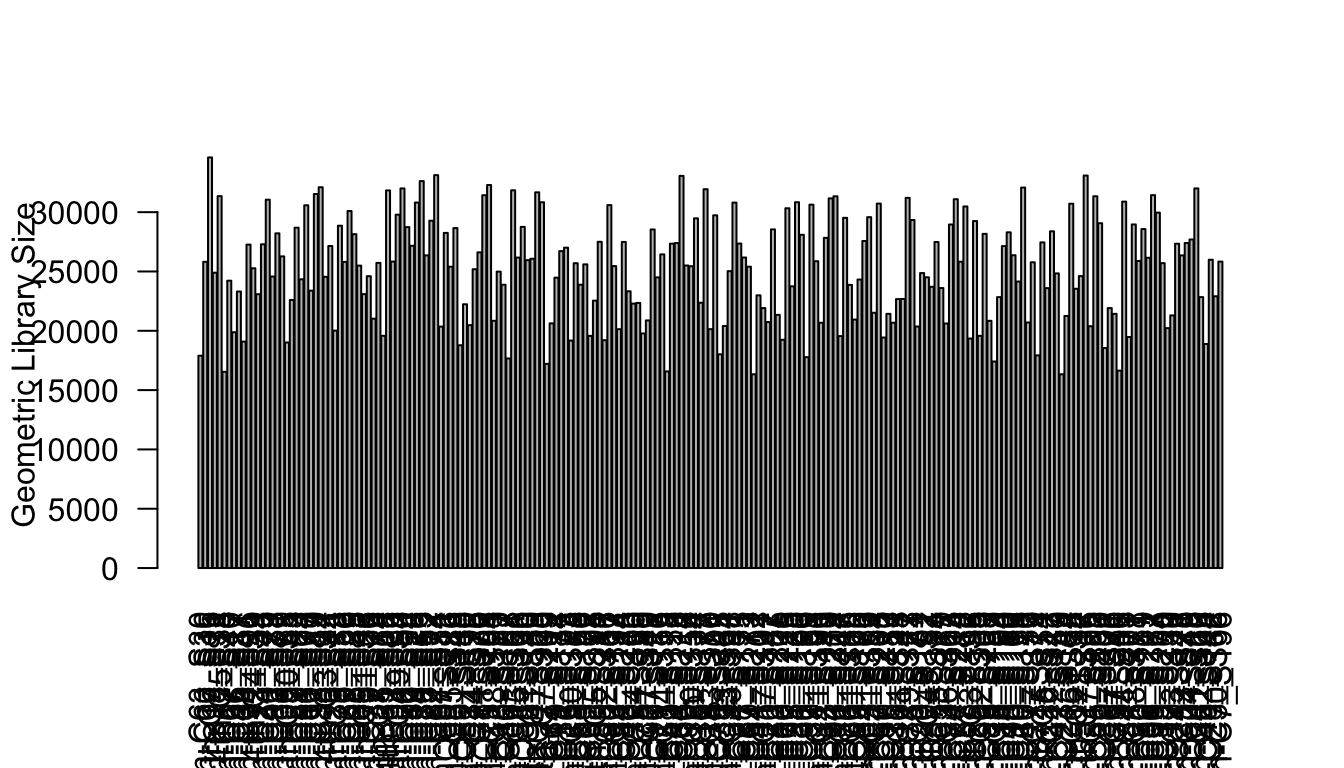

lcounts <- log(counts + 1)
# PC1 and Geometric library size correlation
pc1 = irlba(lcounts - rowMeans(lcounts), 1)$v[,1] ## partial SVD
cor(Geo_Lib, pc1)

[1] -0.9796015

Run tSNE to cluster islet cells.

For comparison purposes, we applied tSNE on read counts of all genes. We used the Rtsne R package with default settings for this analyses. Genes are colored with respect to the expression of marker genes.

set.seed(32354388)
tsne.res <- Rtsne(t(lcounts), dims = 2)
plot(tsne.res$Y, main="tSNE", xlab="Dim1", ylab="Dim2", pch=21, 
     col=color.vec[Cell_Type], bg=color.vec[Cell_Type], oma=c(4,4,6,12))
legend("bottomright", levels(Cell_Type), border="white",fill=color.vec, bty="n")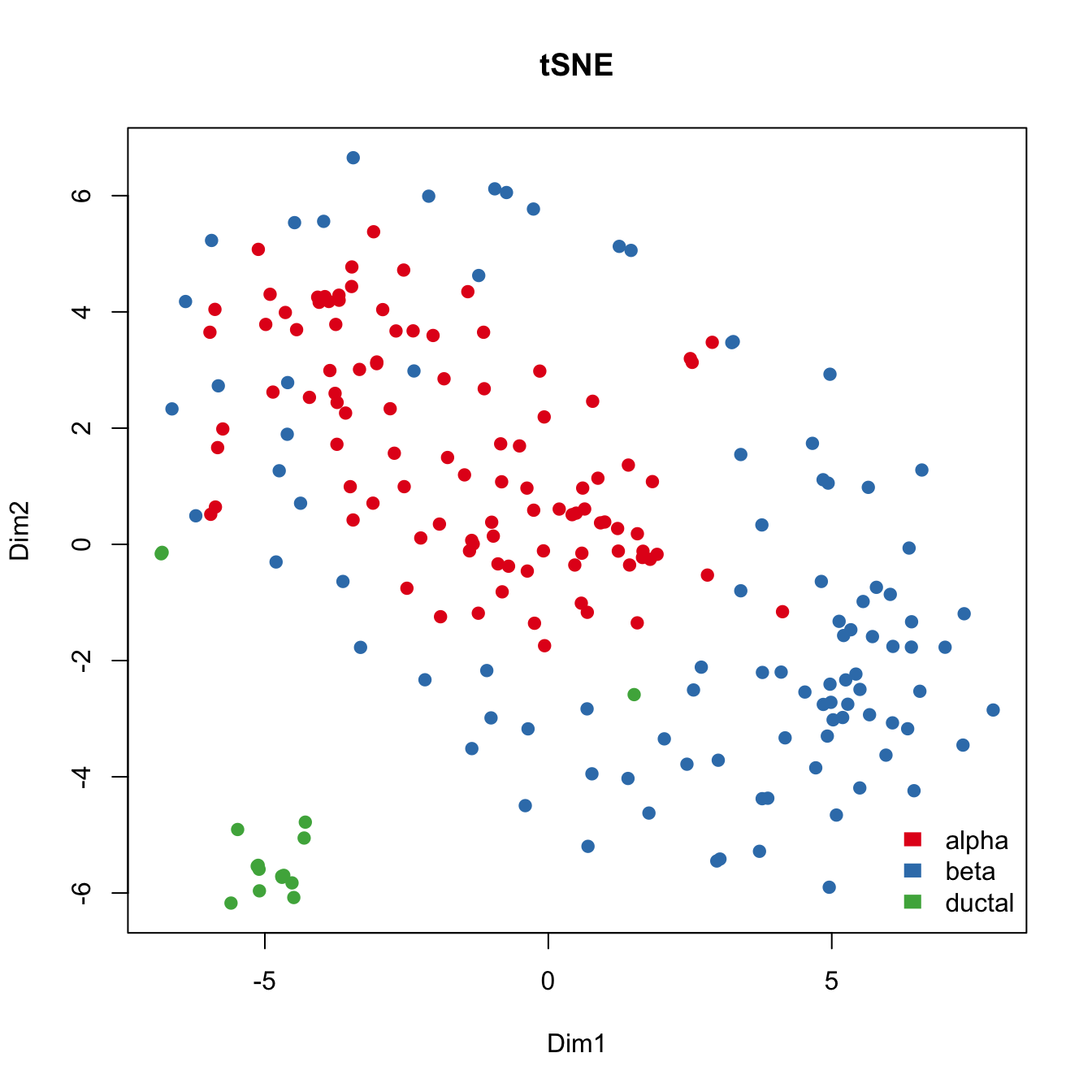

Run IA-SVA

Here, we first run IA-SVA using Patient_ID, Batch and Geo_Lib_Size as known factors and identify 5 hidden factors. Since cell type is not used as a known factor in this analyses, IA-SVA will detect the heterogeneity associated with the cell types.

mod <- model.matrix(~Patient_ID+Batch+Geo_Lib)
summ_exp <- SummarizedExperiment(assays = counts)
iasva.res<- iasva(summ_exp, mod[,-1],verbose=FALSE, permute=FALSE, num.sv=5)

IA-SVA running...


SV 1 Detected!


SV 2 Detected!


SV 3 Detected!


SV 4 Detected!


SV 5 Detected!


# of significant surrogate variables: 5

iasva.sv <- iasva.res$sv

#with color-coding based on true cell-type
pairs(iasva.sv, main="IA-SVA", pch=21, col=color.vec[Cell_Type],
      bg=color.vec[Cell_Type], oma=c(4,4,6,14))
legend("right", levels(Cell_Type), border="white", fill=color.vec, bty="n")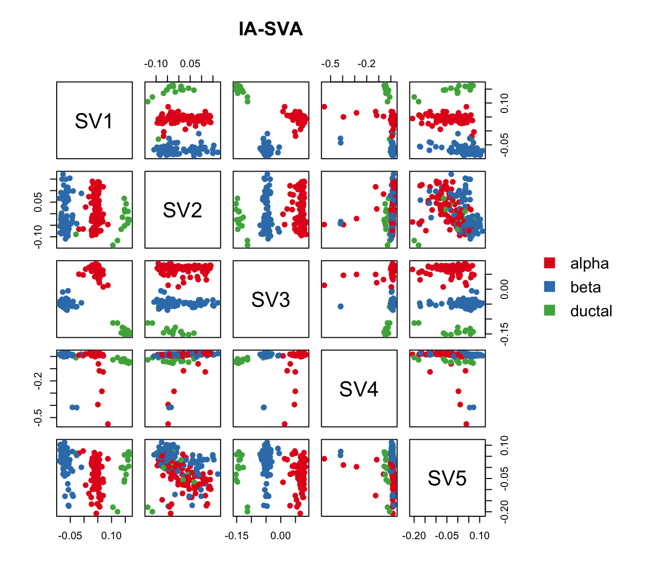

cor(Num_Detected_Genes, iasva.sv)

             SV1        SV2         SV3        SV4       SV5
[1,] -0.06492242 -0.6767266 -0.09183223 -0.1677585 0.7053465

cor(Geo_Lib, iasva.sv)

            SV1        SV2       SV3        SV4       SV5
[1,] -0.2044236 -0.7212868 -0.275179 -0.1841835 0.7725583

corrplot(cor(iasva.sv))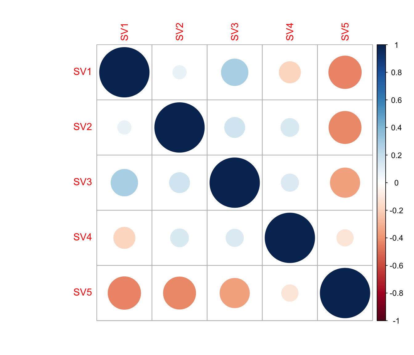

Find marker genes for SV1 and SV3.

Here, using the find_markers() function we find marker genes significantly associated with SV1 and SV3 (multiple testing adjusted p-value < 0.05, default significance cutoff, a high R-squared value: R-squared > 0.4).

# try different R2 thresholds
pdf("Clustering_analyses_figure4_islets_sv1_3.pdf")
r2.results <- study_R2(summ_exp, iasva.sv,selected.svs=c(1,3), no.clusters=3)

# of markers (SV1): 682

# of markers (SV3): 534

total # of unique markers: 979

# of markers (SV1): 357

# of markers (SV3): 281

total # of unique markers: 519

# of markers (SV1): 207

# of markers (SV3): 161

total # of unique markers: 309

# of markers (SV1): 123

# of markers (SV3): 99

total # of unique markers: 192

# of markers (SV1): 78

# of markers (SV3): 62

total # of unique markers: 129

# of markers (SV1): 44

# of markers (SV3): 37

total # of unique markers: 79

# of markers (SV1): 34

# of markers (SV3): 26

total # of unique markers: 58

# of markers (SV1): 25

# of markers (SV3): 20

total # of unique markers: 44

# of markers (SV1): 19

# of markers (SV3): 14

total # of unique markers: 33

# of markers (SV1): 11

# of markers (SV3): 9

total # of unique markers: 20

# of markers (SV1): 8

# of markers (SV3): 7

total # of unique markers: 15

# of markers (SV1): 4

# of markers (SV3): 7

total # of unique markers: 11

# of markers (SV1): 2

# of markers (SV3): 5

total # of unique markers: 7

# of markers (SV1): 2

# of markers (SV3): 3

total # of unique markers: 5

# of markers (SV1): 1

# of markers (SV3): 3

total # of unique markers: 4

# of markers (SV1): 0

# of markers (SV3): 1

total # of unique markers: 1

# of markers (SV1): 0

# of markers (SV3): 0

total # of unique markers: 0

dev.off()

quartz_off_screen 
                2

marker.counts <- find_markers(summ_exp, as.matrix(iasva.sv[,c(1,3)])
                              , rsq.cutoff = 0.4)

# of markers (SV1): 34

# of markers (SV3): 26

total # of unique markers: 58

nrow(marker.counts)

[1] 58

anno.col <- data.frame(Cell_Type=Cell_Type)
rownames(anno.col) <- colnames(marker.counts)
head(anno.col)

            Cell_Type
4th-C63_S30     alpha
4th-C66_S36     alpha
4th-C7_S15       beta
4th-C18_S31     alpha
4th-C5_S8        beta
4th-C57_S18     alpha

cell.type.col <- color.vec[1:3]
names(cell.type.col) <- c("alpha","beta","ductal")
anno.colors <- list(Cell_Type=cell.type.col)

pheatmap(log(marker.counts+1), show_colnames =FALSE, 
         clustering_method = "ward.D2", cutree_cols = 3, 
         annotation_col = anno.col, annotation_colors = anno.colors)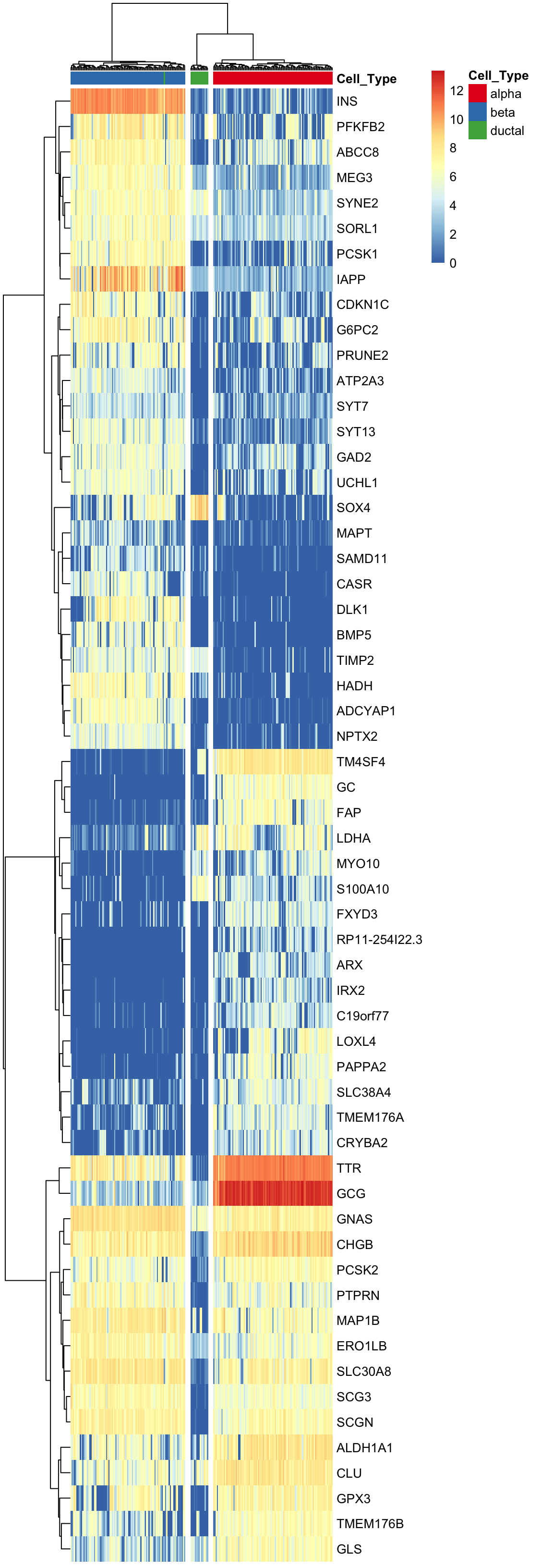

In the case of islet cells, marker genes are well established and IA-SVA did an excellent job of redefining these markers along with some other highly informative genes. Therefore, IA-SVA can be effectively used to uncover heterogeneity associated with cell types and can reveal genes that are expressed in a cell-specific manner.

Find marker genes for SV4.

Here, using the find_markers() function we find marker genes significantly associated with SV4 (multiple testing adjusted p-value < 0.05, default significance cutoff, a high R-squared value: R-squared > 0.3).

marker.counts.SV4 <- find_markers(summ_exp, as.matrix(iasva.sv[,c(4)]),
                                  rsq.cutoff = 0.3)

# of markers (): 94

total # of unique markers: 94

nrow(marker.counts.SV4)

[1] 94

anno.col <- data.frame(SV4=iasva.sv[,4])
rownames(anno.col) <- colnames(marker.counts)
head(anno.col)

                     SV4
4th-C63_S30  0.022045049
4th-C66_S36  0.006979656
4th-C7_S15   0.014475352
4th-C18_S31  0.012836294
4th-C5_S8    0.009518166
4th-C57_S18 -0.126329593

pheatmap(log(marker.counts.SV4+1), show_colnames =FALSE, 
         clustering_method = "ward.D2", cutree_cols = 2,
         annotation_col = anno.col)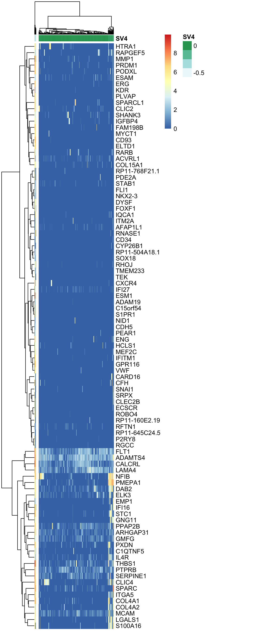

Run tSNE post IA-SVA, i.e., run tSNE on marker genes for SV1 and SV2 obtained from IA-SVA.

Here, we apply tSNE on the marker genes for SV1 and SV2

set.seed(344588)
tsne.res.iasva <- Rtsne(unique(t(log(marker.counts+1))), dims = 2)
plot(tsne.res.iasva$Y, main="IA-SVA + tSNE", xlab="Dimension 1",
     ylab="Dimension 2", pch=21, col=color.vec[Cell_Type],
     bg=color.vec[Cell_Type], oma=c(4,4,6,12))
legend("topright", levels(Cell_Type), border="white", fill=color.vec, bty="n")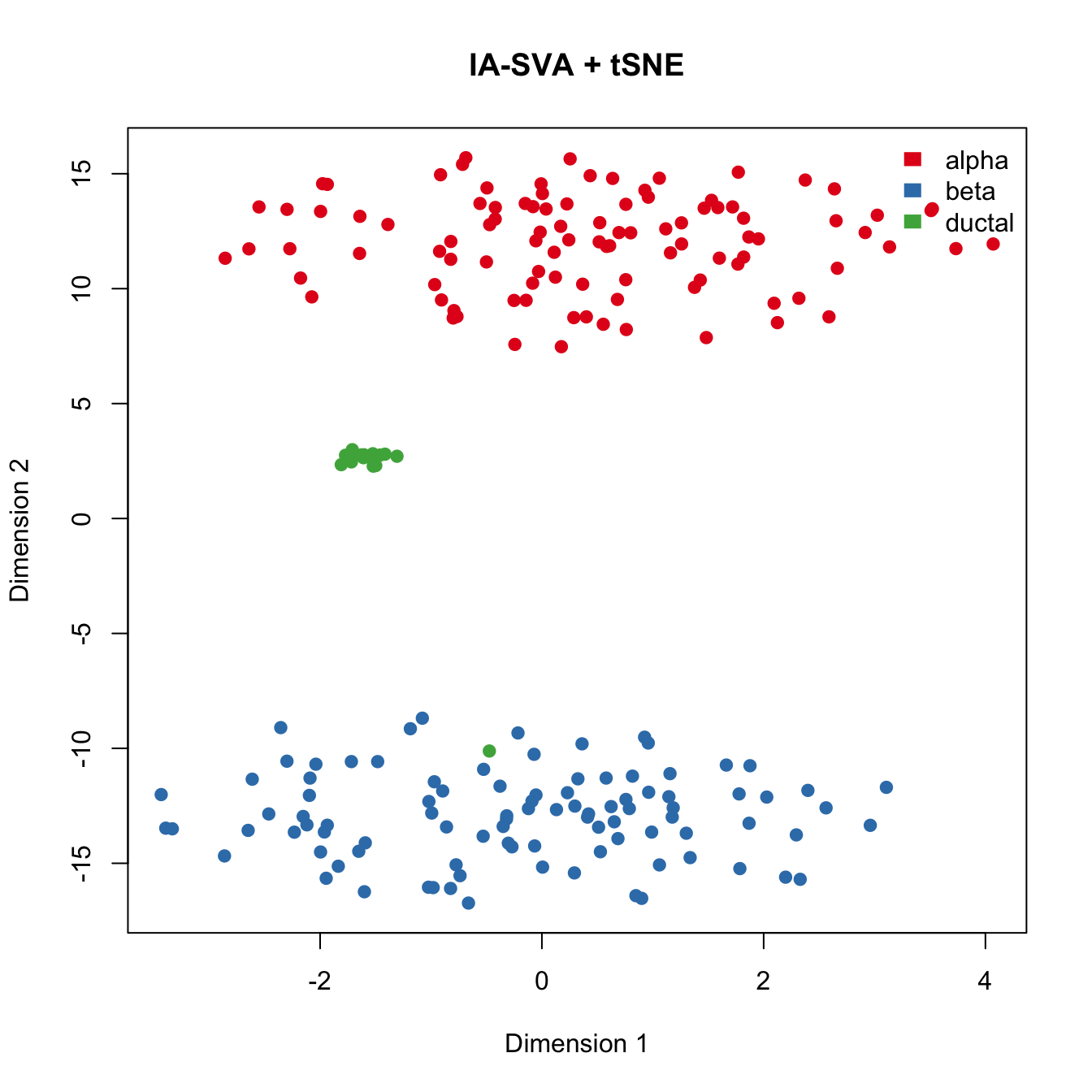

tSNE conducted on genes selected via IA-SVA very clearly seperates cells into their corresponding cell types. Moreover, this analyses also revealed one cell (green cell clustered together with blue cells) that is potentially mislabeled in the original analyses.

Run CellView algorithm to visualize the data.

# specify gene number to select for
gene_num <- 1000
# calcuclate dispersion
row.var <- apply(lcounts,1,sd)**2
row.mean <- apply(lcounts,1,mean)
dispersion <- row.var/row.mean

# generate sequence of bins
bins <- seq(from = min(row.mean), to = max(row.mean), length.out = 20)

# sort mean expression data into the bins
bin.exp <- row.mean
# sort the values
bin.sort <- sort(bin.exp, decreasing = FALSE)
# vector of bin assignment
cuts <- cut(x = bin.exp, breaks = bins, labels = FALSE)
# find which are NA and change to zero
na.ids <- which(is.na(cuts) == TRUE)
cuts[na.ids] <- 0

# create an empty vector for overdispersion
overdispersion <- NULL

# for each gene and bin index, calculate median, mad, and then normalized dispersion
# first loop through length of bins found
for (k in 1:length(names(table(cuts)))) {
  # find index of bins
  bin.id <- which(cuts == names(table(cuts))[k])
  # median of all genes in the bin
  median.bin <- median(dispersion[bin.id], na.rm = TRUE)
  # calculate mad (median absolute deviation)
  mad.bin <- mad(dispersion[bin.id])
  # calculate norm dispersion for each gene
  for (m in 1:length(bin.id)) {
    norm.dispersion <- abs(dispersion[bin.id[m]] - median.bin)/mad.bin
    overdispersion <- c(overdispersion, norm.dispersion) 
  }
}

# remove nans 
overdis.na <- which(is.na(overdispersion) == TRUE)
if (length(overdis.na) > 0) {
  overdis.filt <- overdispersion[-overdis.na]
} else {
  overdis.filt <- overdispersion
}

# plot mean expression vs overdisperssion
ids <- which(names(overdis.filt) %in% names(row.mean))
plot(row.mean[ids], overdis.filt)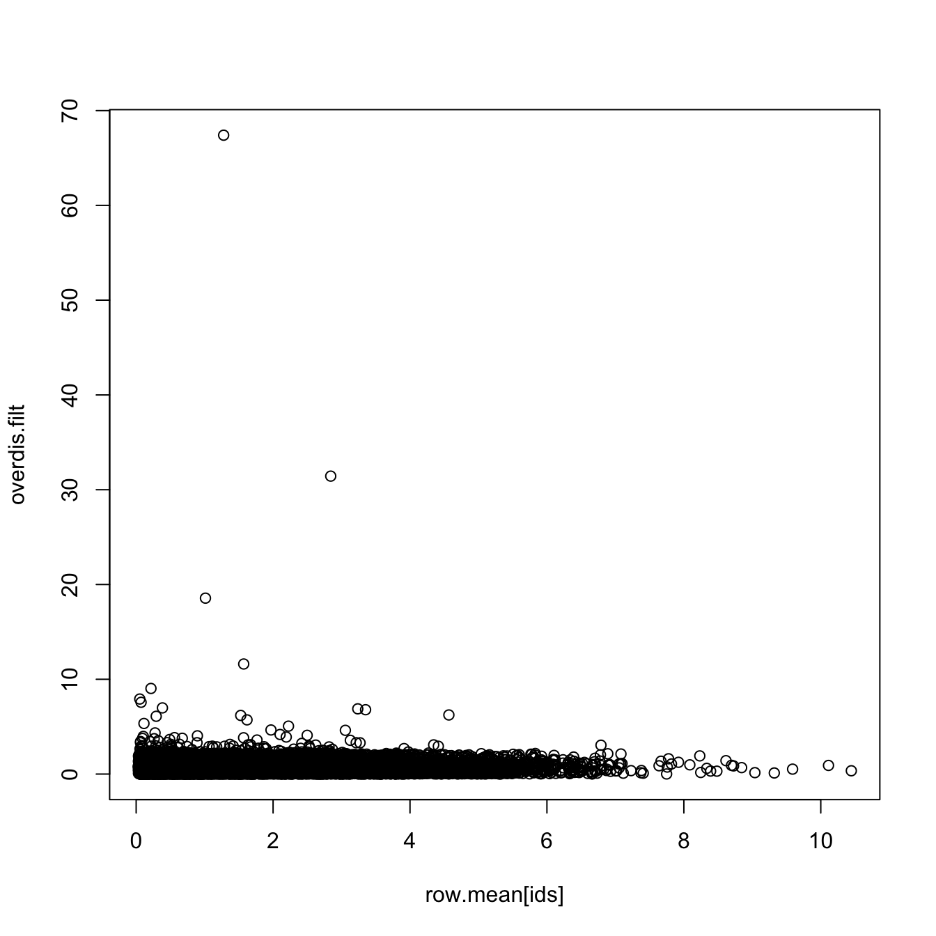

# Do t-sne using top over-dispersed genes (apply mean expression filter too)
rank.ov <- order(overdis.filt, decreasing = TRUE)
ov.genes <- names(overdis.filt[rank.ov[1:gene_num]])
log.sel <- lcounts[ov.genes,]

all1 <- t(log.sel)
# Remove groups that are all zeros
df <- all1[,apply(all1, 2, var, na.rm=TRUE) != 0]

set.seed(34544532)
rtsne_out <- Rtsne(as.matrix(df), dims = 3)

# Set rownames of matrix to tsne matrix
rownames(rtsne_out$Y) <- rownames(df)

tsne.cellview <- rtsne_out$Y

plot(tsne.cellview[,c(1,2)], main="CellView", xlab="Dimension 1", 
     ylab="Dimension 2",pch=21, col=color.vec[Cell_Type], 
     bg=color.vec[Cell_Type], oma=c(4,4,6,12))
legend("topright", levels(Cell_Type), border="white", fill=color.vec, bty="n")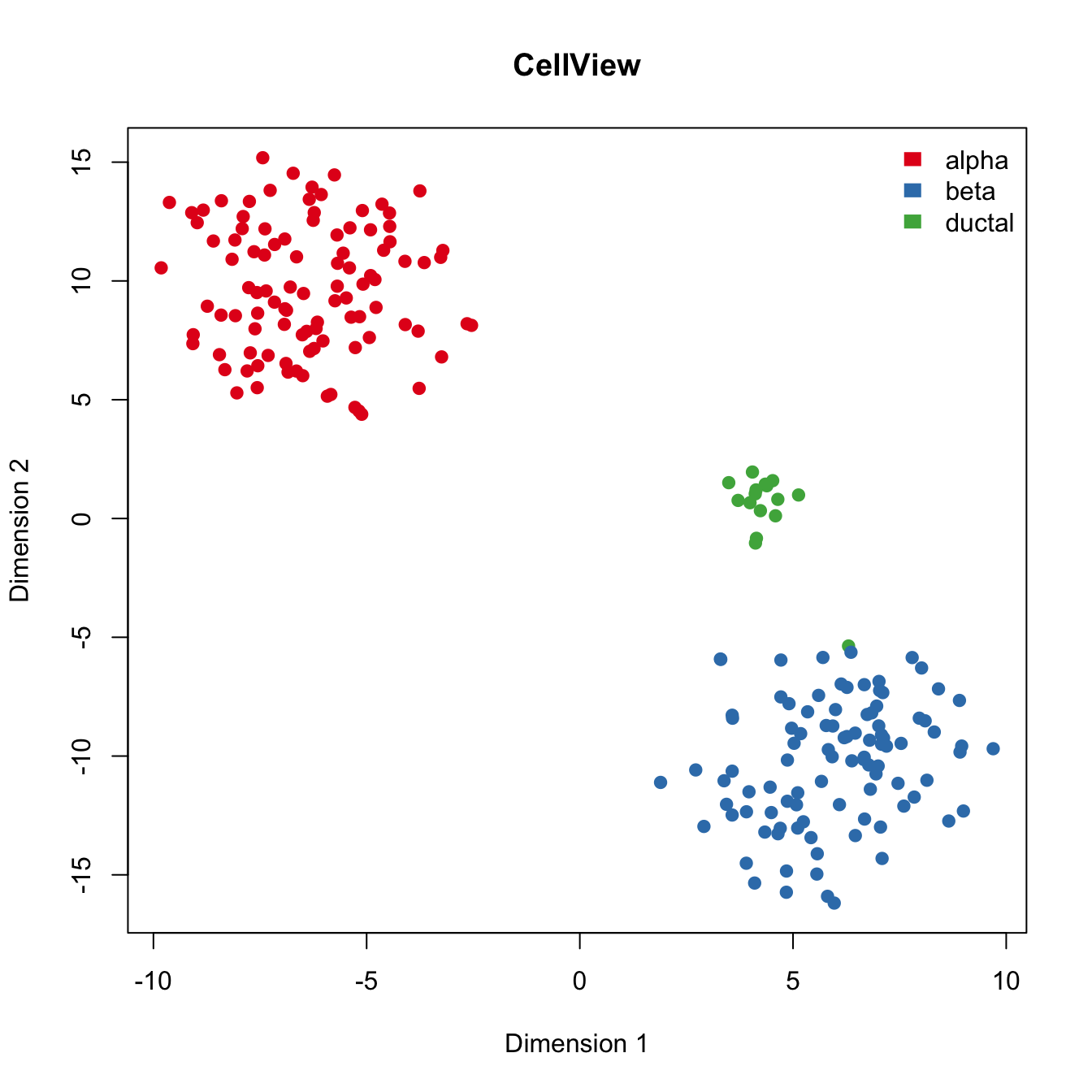

Run Seurat to reduce dimensionality and visualize islet cells

set.seed(12344)
seurat.obj <- CreateSeuratObject(raw.data=raw.counts, 
                                 min.cells=3, min.genes=200, project="Seurat_Comp")

names(Patient_ID) <- rownames(seurat.obj@meta.data)
seurat.obj <- AddMetaData(object = seurat.obj, 
                          metadata = Patient_ID, col.name = "patient.id")
names(Batch) <- rownames(seurat.obj@meta.data)
seurat.obj <- AddMetaData(object = seurat.obj, 
                          metadata = Batch, col.name = "batch")
names(Geo_Lib) <- rownames(seurat.obj@meta.data)
seurat.obj <- AddMetaData(object = seurat.obj, 
                          metadata = Geo_Lib, col.name = "geo.lib")

# Normalizing the data
seurat.obj <- NormalizeData(object = seurat.obj,
                            normalization.method = "LogNormalize", 
                            scale.factor = median(colSums(raw.counts)))

# Detection of variable genes across the single cells
seurat.obj <- FindVariableGenes(object = seurat.obj, 
                                mean.function = ExpMean, dispersion.function = LogVMR, 
    x.low.cutoff = 0.0125, x.high.cutoff = 3, y.cutoff = 0.5)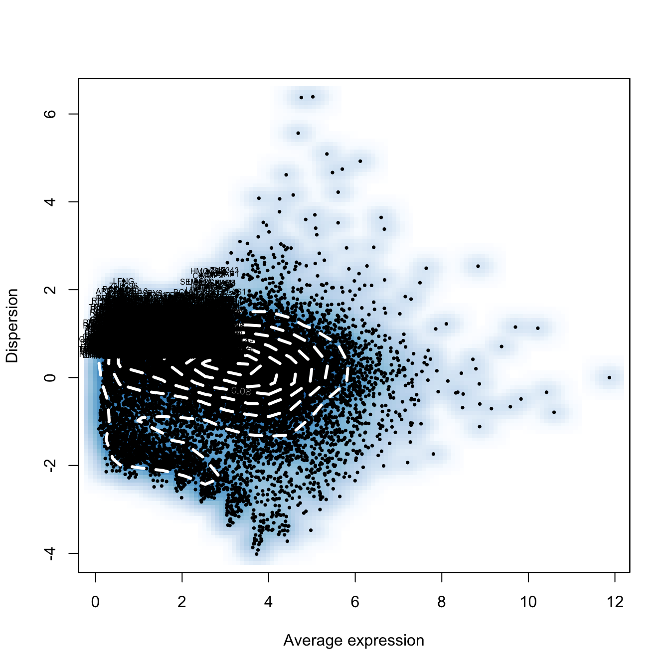

length(x = seurat.obj@var.genes)

[1] 2933

# Scaling the data and removing unwanted sources of variation
seurat.obj <- ScaleData(object = seurat.obj, 
                        vars.to.regress = c("patient.id", "batch", "geo.lib"))

Regressing out: patient.id, batch, geo.lib


Time Elapsed:  9.59692406654358 secs

Scaling data matrix

# Perform linear dimensional reduction
seurat.obj <- RunPCA(object = seurat.obj, 
                     pc.genes = seurat.obj@var.genes, 
                     do.print = TRUE, pcs.print = 1:5, 
                     genes.print = 5)

[1] "PC1"
[1] "CCDC108"       "SGIP1"         "MBD5"          "RP11-222A11.1"
[5] "GLRA3"        
[1] ""
[1] "DEFB1" "VTCN1" "PKHD1" "ITGB6" "PROM1"
[1] ""
[1] ""
[1] "PC2"
[1] "ELTD1"  "GPR116" "ERG"    "VWF"    "DYSF"  
[1] ""
[1] "VTCN1"  "DEFB1"  "PKHD1"  "ITGB6"  "LGALS4"
[1] ""
[1] ""
[1] "PC3"
[1] "PAQR4"   "SLITRK6" "BUB1B"   "MTFR2"   "TFAP2A" 
[1] ""
[1] "GCKR"         "LYPD6B"       "LGALS4"       "C6orf222"    
[5] "RP4-534N18.2"
[1] ""
[1] ""
[1] "PC4"
[1] "BUB1"   "ASPM"   "KIFC1"  "RAD51"  "DEPDC1"
[1] ""
[1] "SLIT2"  "COL5A1" "TFAP2A" "RUNX2"  "SFRP1" 
[1] ""
[1] ""
[1] "PC5"
[1] "FHL3"   "FGG"    "MAMLD1" "PRKCG"  "KRT222"
[1] ""
[1] "GLRA1"   "EPB41L2" "ADRA2A"  "TET1"    "DACH2"  
[1] ""
[1] ""

# Run tSNE (Spectral tSNE)
set.seed(8883)
seurat.obj <- RunTSNE(object = seurat.obj, dims.use = 1:5, do.fast = TRUE)

# tSNE plot with color-coding of true cell types
plot(seurat.obj@dr$tsne@cell.embeddings[,c(1,2)], 
     main="Spectral tSNE (Seurat)", xlab="Dimension 1",
     ylab="Dimension 2",pch=21, col=color.vec[Cell_Type], 
     bg=color.vec[Cell_Type], oma=c(4,4,6,12))
legend("topleft", levels(Cell_Type), border="white", fill=color.vec, bty="n")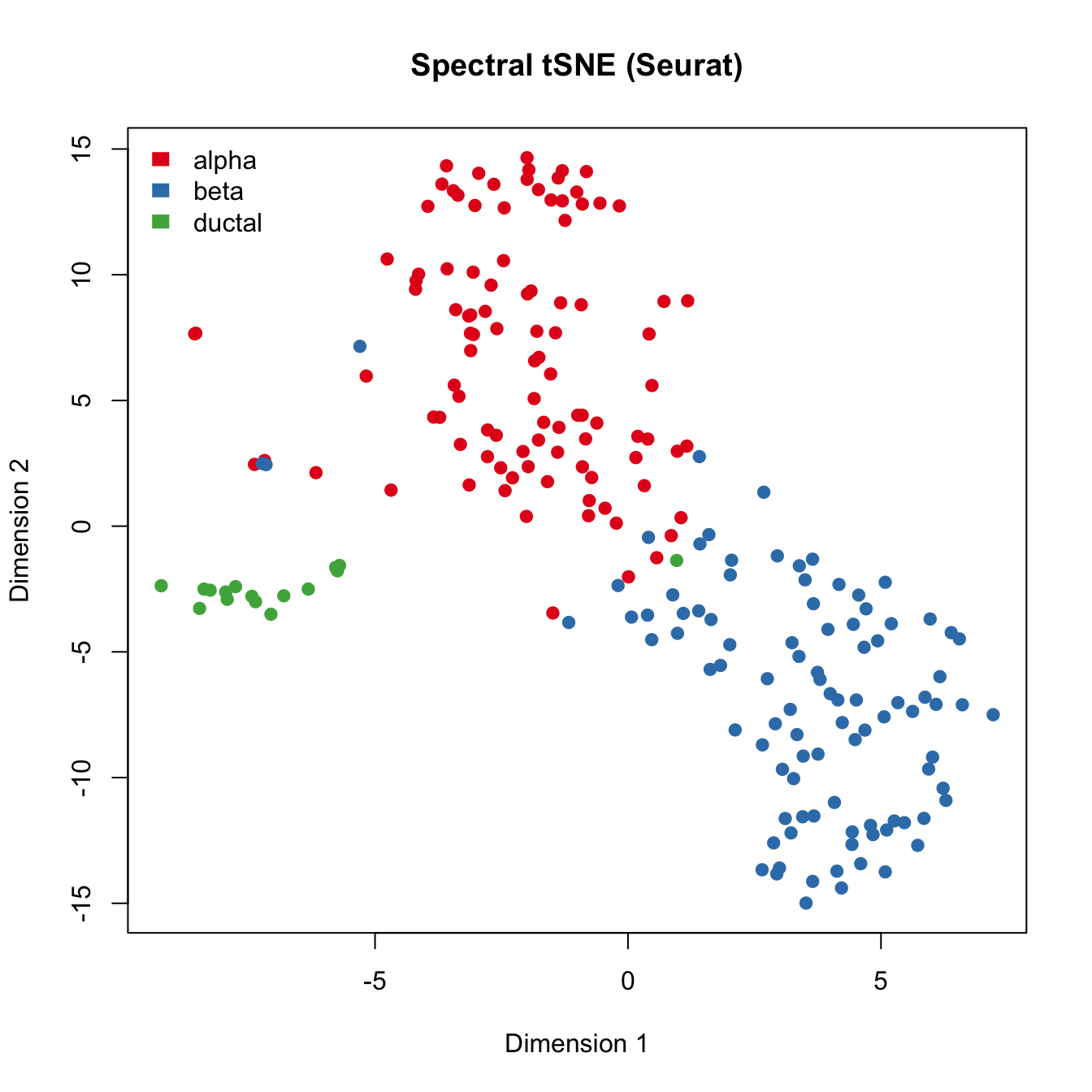

pdf(file="output/Lawlor_Islets_3Cells_tSNE_IA-SVA_Fig4AB.pdf", width=9, height=5)
layout(matrix(c(1,2), nrow=1, ncol=2, byrow=TRUE))
plot(tsne.res$Y, main="tSNE", xlab="Dimension 1", 
     ylab="Dimension 2", pch=21, col=color.vec[Cell_Type],
     bg=color.vec[Cell_Type])
legend("topleft", levels(Cell_Type), border="white",
       fill=color.vec, bty="n")
plot(tsne.res.iasva$Y, main="IA-SVA + tSNE", xlab="Dimension 1", 
     ylab="Dimension 2", pch=21, col=color.vec[Cell_Type], 
     bg=color.vec[Cell_Type])
legend("topright", levels(Cell_Type), border="white", 
       fill=color.vec, bty="n")
dev.off()

quartz_off_screen 
                2

anno.col <- data.frame(Cell_Type=Cell_Type)
rownames(anno.col) <- colnames(marker.counts)
head(anno.col)

            Cell_Type
4th-C63_S30     alpha
4th-C66_S36     alpha
4th-C7_S15       beta
4th-C18_S31     alpha
4th-C5_S8        beta
4th-C57_S18     alpha

cell.type.col <- color.vec[1:3]
names(cell.type.col) <- c("alpha","beta","ductal")
anno.colors <- list(Cell_Type=cell.type.col)

pheatmap(log(marker.counts+1), show_colnames =FALSE, 
         clustering_method = "ward.D2", cutree_cols = 3, 
         annotation_col = anno.col, annotation_colors = anno.colors,
         filename="output/Lawlor_Islets_3Cells_IASVA_SV1SV3_rsqcutoff0.3_pheatmap_iasvaV0.95_Figure4_C.pdf",
         width=6, height=17)

pdf(file="output/Lawlor_Islets_3Cells_IASVA_pairs4SVs_iasvaV0.95_black_FigS6.pdf",
    width=4, height=4)
pairs(iasva.sv[,1:4], pch=21, col="black", bg="black")
dev.off()

quartz_off_screen 
                2

pdf(file="output/Lawlor_Islets_3Cells_IASVA_pairs4SVs_iasvaV0.95_color_FigS6.pdf", 
    width=4, height=4)
pairs(iasva.sv[,1:4], pch=21, col=color.vec[Cell_Type], 
      bg=color.vec[Cell_Type])
dev.off()

quartz_off_screen 
                2

## 1,2
pdf(file="output/Lawlor_Islets_3Cells_CellView_Seurat_FigS.pdf", width=9, height=5)
layout(matrix(c(1,2), nrow=1, ncol=2, byrow=TRUE))
plot(tsne.cellview[,c(1,2)], main="CellView", xlab="Dimension 1",
     ylab="Dimension 2",pch=21, col=color.vec[Cell_Type],
     bg=color.vec[Cell_Type], oma=c(4,4,6,12))
legend("topright", levels(Cell_Type), border="white",
       fill=color.vec, bty="n")
plot(seurat.obj@dr$tsne@cell.embeddings[,c(1,2)], 
     main="Spectral tSNE (Seurat)", xlab="Dimension 1", 
     ylab="Dimension 2",pch=21, col=color.vec[Cell_Type], 
     bg=color.vec[Cell_Type], oma=c(4,4,6,12))
legend("topleft", levels(Cell_Type), border="white", 
       fill=color.vec, bty="n")
dev.off()

quartz_off_screen 
                2

write.table(as.data.frame(rownames(marker.counts)), 
            file="output/Lawlor_Islets_3Cells_SV1_SV3_Cell_Type_Genes_rsqcutoff0.3.txt",
            quote=F, row.names=F, col.names=F, sep=" ")

write.table(as.data.frame(rownames(marker.counts.SV4)), 
            file="output/Lawlor_Islets_3Cells_SV4_Genes_rsqcutoff0.3.txt", quote=F,
            row.names=F, col.names=F, sep=" ")

anno.col <- data.frame(SV4=iasva.sv[,4])
rownames(anno.col) <- colnames(marker.counts)
head(anno.col)

                     SV4
4th-C63_S30  0.022045049
4th-C66_S36  0.006979656
4th-C7_S15   0.014475352
4th-C18_S31  0.012836294
4th-C5_S8    0.009518166
4th-C57_S18 -0.126329593

pheatmap(log(marker.counts.SV4+1), show_colnames =FALSE, 
         clustering_method = "ward.D2", cutree_cols = 2, 
         annotation_col = anno.col,
         filename="output/Lawlor_Islets_3Cells_IASVA_SV4_rsqcutoff0.3_pheatmap_iasvaV0.95.pdf",
         width=8, height=14)

Session information

sessionInfo()

R version 3.5.0 (2018-04-23)
Platform: x86_64-apple-darwin15.6.0 (64-bit)
Running under: macOS Sierra 10.12.6

Matrix products: default
BLAS: /Library/Frameworks/R.framework/Versions/3.5/Resources/lib/libRblas.0.dylib
LAPACK: /Library/Frameworks/R.framework/Versions/3.5/Resources/lib/libRlapack.dylib

locale:
[1] en_US.UTF-8/en_US.UTF-8/en_US.UTF-8/C/en_US.UTF-8/en_US.UTF-8

attached base packages:
[1] parallel  stats4    stats     graphics  grDevices utils     datasets 
[8] methods   base     

other attached packages:
 [1] SummarizedExperiment_1.10.1 DelayedArray_0.6.1         
 [3] BiocParallel_1.14.2         matrixStats_0.53.1         
 [5] Biobase_2.40.0              GenomicRanges_1.32.3       
 [7] GenomeInfoDb_1.16.0         IRanges_2.14.10            
 [9] S4Vectors_0.18.3            BiocGenerics_0.26.0        
[11] RColorBrewer_1.1-2          DescTools_0.99.24          
[13] corrplot_0.84               pheatmap_1.0.10            
[15] Rtsne_0.13                  dbscan_1.1-2               
[17] Seurat_2.3.2                cowplot_0.9.2              
[19] ggplot2_2.2.1.9000          iasvaExamples_1.0.0        
[21] iasva_0.99.3                irlba_2.3.2                
[23] Matrix_1.2-14              

loaded via a namespace (and not attached):
  [1] snow_0.4-2             backports_1.1.2        Hmisc_4.1-1           
  [4] workflowr_1.0.1        VGAM_1.0-5             plyr_1.8.4            
  [7] igraph_1.2.1           lazyeval_0.2.1         splines_3.5.0         
 [10] digest_0.6.15          foreach_1.4.4          htmltools_0.3.6       
 [13] lars_1.2               gdata_2.18.0           magrittr_1.5          
 [16] checkmate_1.8.5        cluster_2.0.7-1        mixtools_1.1.0        
 [19] ROCR_1.0-7             sfsmisc_1.1-2          recipes_0.1.3         
 [22] gower_0.1.2            dimRed_0.1.0           R.utils_2.6.0         
 [25] colorspace_1.3-2       dplyr_0.7.5            jsonlite_1.5          
 [28] RCurl_1.95-4.10        bindr_0.1.1            zoo_1.8-2             
 [31] survival_2.42-3        iterators_1.0.9        ape_5.1               
 [34] glue_1.2.0             DRR_0.0.3              gtable_0.2.0          
 [37] ipred_0.9-6            zlibbioc_1.26.0        XVector_0.20.0        
 [40] kernlab_0.9-26         ddalpha_1.3.3          prabclus_2.2-6        
 [43] DEoptimR_1.0-8         abind_1.4-5            scales_0.5.0          
 [46] mvtnorm_1.0-8          Rcpp_0.12.17           dtw_1.20-1            
 [49] metap_0.9              htmlTable_1.12         tclust_1.4-1          
 [52] magic_1.5-8            reticulate_1.8         bit_1.1-14            
 [55] proxy_0.4-22           foreign_0.8-70         mclust_5.4            
 [58] SDMTools_1.1-221       Formula_1.2-3          tsne_0.1-3            
 [61] lava_1.6.1             prodlim_2018.04.18     htmlwidgets_1.2       
 [64] FNN_1.1                gplots_3.0.1           fpc_2.1-11            
 [67] acepack_1.4.1          modeltools_0.2-21      ica_1.0-2             
 [70] manipulate_1.0.1       pkgconfig_2.0.1        R.methodsS3_1.7.1     
 [73] flexmix_2.3-14         nnet_7.3-12            caret_6.0-80          
 [76] tidyselect_0.2.4       rlang_0.2.1            reshape2_1.4.3        
 [79] munsell_0.4.3          tools_3.5.0            ranger_0.10.1         
 [82] pls_2.6-0              ggridges_0.5.0         broom_0.4.4           
 [85] evaluate_0.10.1        geometry_0.3-6         stringr_1.3.1         
 [88] yaml_2.1.19            bit64_0.9-7            ModelMetrics_1.1.0    
 [91] knitr_1.20             fitdistrplus_1.0-9     robustbase_0.93-0     
 [94] caTools_1.17.1         purrr_0.2.5            RANN_2.5.1            
 [97] bindrcpp_0.2.2         pbapply_1.3-4          nlme_3.1-137          
[100] whisker_0.3-2          R.oo_1.22.0            RcppRoll_0.3.0        
[103] hdf5r_1.0.0            compiler_3.5.0         rstudioapi_0.7        
[106] png_0.1-7              tibble_1.4.2           stringi_1.2.2         
[109] lattice_0.20-35        trimcluster_0.1-2      psych_1.8.4           
[112] diffusionMap_1.1-0     pillar_1.2.3           lmtest_0.9-36         
[115] data.table_1.11.4      bitops_1.0-6           R6_2.2.2              
[118] latticeExtra_0.6-28    KernSmooth_2.23-15     gridExtra_2.3         
[121] codetools_0.2-15       boot_1.3-20            MASS_7.3-50           
[124] gtools_3.5.0           assertthat_0.2.0       CVST_0.2-2            
[127] rprojroot_1.3-2        withr_2.1.2            mnormt_1.5-5          
[130] GenomeInfoDbData_1.1.0 expm_0.999-2           diptest_0.75-7        
[133] doSNOW_1.0.16          grid_3.5.0             rpart_4.1-13          
[136] timeDate_3043.102      tidyr_0.8.1            class_7.3-14          
[139] rmarkdown_1.9          segmented_0.5-3.0      git2r_0.21.0          
[142] lubridate_1.7.4        scatterplot3d_0.3-41   base64enc_0.1-3

This reproducible R Markdown analysis was created with workflowr 1.0.1