Reviewer 2 Simulation
Donghyung Lee
2018-08-27
- The reviewer 2’s simulation #1 with weak unknown factor.
- The reviewer 2’s simulation #2 with stronger effect size.
- Several issues in the simulation studies suggested by the reviewer #2
- Corrected simulation with low correlation btw known and hidden factors
- Corrected Simulation with high correlation btw known and hidden factors with stronger effect sizes
- More challenging scenario.
- Session information
Last updated: 2018-08-27
workflowr checks: (Click a bullet for more information)-
✔ R Markdown file: up-to-date
Great! Since the R Markdown file has been committed to the Git repository, you know the exact version of the code that produced these results.
-
✔ Environment: empty
Great job! The global environment was empty. Objects defined in the global environment can affect the analysis in your R Markdown file in unknown ways. For reproduciblity it’s best to always run the code in an empty environment.
-
✔ Seed:
set.seed(20180731)The command
set.seed(20180731)was run prior to running the code in the R Markdown file. Setting a seed ensures that any results that rely on randomness, e.g. subsampling or permutations, are reproducible. -
✔ Session information: recorded
Great job! Recording the operating system, R version, and package versions is critical for reproducibility.
-
Great! You are using Git for version control. Tracking code development and connecting the code version to the results is critical for reproducibility. The version displayed above was the version of the Git repository at the time these results were generated.✔ Repository version: 492eafb
Note that you need to be careful to ensure that all relevant files for the analysis have been committed to Git prior to generating the results (you can usewflow_publishorwflow_git_commit). workflowr only checks the R Markdown file, but you know if there are other scripts or data files that it depends on. Below is the status of the Git repository when the results were generated:
Note that any generated files, e.g. HTML, png, CSS, etc., are not included in this status report because it is ok for generated content to have uncommitted changes.Ignored files: Ignored: .DS_Store Ignored: .Rhistory Ignored: .Rproj.user/ Ignored: data/.DS_Store Ignored: docs/.DS_Store Ignored: docs/figure/.DS_Store Ignored: inst/.DS_Store Ignored: inst/doc/.DS_Store Ignored: output/.DS_Store Ignored: vignettes/.DS_Store
Expand here to see past versions:
| File | Version | Author | Date | Message |
|---|---|---|---|---|
| Rmd | 492eafb | dleelab | 2018-08-27 | figure number changed |
| Rmd | e042edf | dleelab | 2018-08-27 | figure updated |
| html | 5e29c04 | dleelab | 2018-08-22 | reviewer2 sim updated. |
| Rmd | 17ebb03 | dleelab | 2018-08-22 | text edit |
| Rmd | fa4ce46 | dleelab | 2018-08-21 | figure changed |
| Rmd | cf73dbb | dleelab | 2018-08-21 | reviewer2 sim updated |
| Rmd | c241b04 | dleelab | 2018-08-03 | added |
| html | c241b04 | dleelab | 2018-08-03 | added |
The reviewer 2’s simulation #1 with weak unknown factor.
# Setting up the known and unknown factors.
set.seed(10000)
known <- runif(1000)
unknown <- runif(1000, 0, 0.1) # weak unknown factor

# Generating Poisson count data from log-normal means.
ngenes <- 5000
known.effect <- rnorm(ngenes, sd=2)
unknown.effect <- rnorm(ngenes, sd=2)
mat <- outer(known.effect, known) + outer(unknown.effect, unknown) + 2 # to get decent-sized counts

counts <- matrix(rpois(length(mat), lambda=2^mat), nrow=ngenes)
library(SummarizedExperiment)
se <- SummarizedExperiment(list(counts=counts))

# Running IA-SVA, version 0.99.3.
library(iasva)
design <- model.matrix(~known)
res <- iasva(se, design, num.sv=5, permute = FALSE)
# IA-SVA running...
#
# SV 1 Detected!
#
# SV 2 Detected!
#
# SV 3 Detected!
#
# SV 4 Detected!
#
# SV 5 Detected!
#
# # of significant surrogate variables: 5

cor(res$sv[,1], unknown) # these SVs are not the unknown factor (correlation ~= 0)
# [1] 0.05699341
cor(res$sv[,2], unknown)
# [1] -0.1317231
cor(res$sv[,3], unknown)
# [1] 0.06301151
cor(res$sv[,4], unknown)
# [1] -0.08444932
cor(res$sv[,5], unknown)
# [1] 0.1239618

cor(res$sv[,1], known) # ... but are instead the known factor (correlation ~= +/-1)
# [1] -0.9988192
cor(res$sv[,2], known)
# [1] 0.9971117
cor(res$sv[,3], known)
# [1] -0.9558875
cor(res$sv[,4], known)
# [1] 0.9982102
cor(res$sv[,5], known)
# [1] -0.9934994

## Compare to just naively taking the first PC of the residual matrix.
library(limma)
#
# Attaching package: 'limma'
# The following object is masked from 'package:BiocGenerics':
#
#     plotMA
resid <- removeBatchEffect(log(assay(se)+1), covariates=known)
pr.out <- prcomp(t(resid), rank.=1)
abs(cor(pr.out$x[,1], unknown)) # close to 1
# [1] 0.9766822
abs(cor(pr.out$x[,1], known)) # close to zero.
# [1] 2.35573e-17

## Compare to SVA
library(sva)
mod1 <- model.matrix(~known)
mod0 <- cbind(mod1[,1])
sva.res = svaseq(counts,mod1,mod0, n.sv=5)$sv
# Number of significant surrogate variables is:  5
# Iteration (out of 5 ):1  2  3  4  5
abs(cor(sva.res[,1], unknown)) # 0.55
# [1] 0.5522043
abs(cor(sva.res[,1], known)) # close to zero.
# [1] 0.04603016

hf.mat1 <- cbind(known, unknown, res$sv[,1], pr.out$x[,1], sva.res[,1])
colnames(hf.mat1) <- c("KF","HF","IASVA","PC1_Residual","SVA")
corrplot.mixed(abs(cor(hf.mat1)), tl.pos="lt")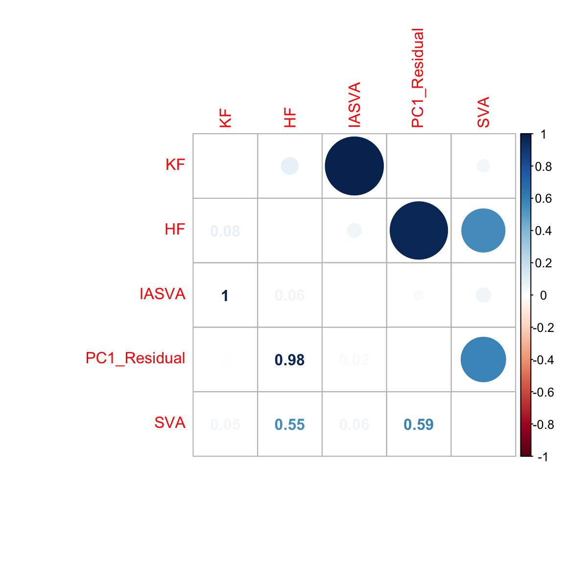
The reviewer 2’s simulation #2 with stronger effect size.
set.seed(10000)

known <- runif(1000)
unknown <- runif(1000)

ngenes <- 5000
known.effect <- rnorm(ngenes, sd=2)
unknown.effect <- rnorm(ngenes, sd=2)
mat <- outer(known.effect, known) + outer(unknown.effect, unknown) + 2 # to get decent-sized counts

counts <- matrix(rpois(length(mat), lambda=2^mat), nrow=ngenes)
library(SummarizedExperiment)
se <- SummarizedExperiment(list(counts=counts))

library(iasva)
design <- model.matrix(~known)
res <- iasva(se, design, num.sv=5, permute = FALSE)
# IA-SVA running...
#
# SV 1 Detected!
#
# SV 2 Detected!
#
# SV 3 Detected!
#
# SV 4 Detected!
#
# SV 5 Detected!
#
# # of significant surrogate variables: 5

cor(res$sv[,1], unknown) # first SV is the unknown factor.
# [1] -0.9960557
cor(res$sv[,2], unknown)
# [1] 0.7637275
cor(res$sv[,3], unknown)
# [1] 0.7564822
cor(res$sv[,4], unknown)
# [1] -0.7629373
cor(res$sv[,5], unknown)
# [1] 0.4760279

cor(res$sv[,1], known)
# [1] -0.004959888
cor(res$sv[,2], known) # but SVs 2-5 are correlated with the known factor...
# [1] -0.7014209
cor(res$sv[,3], known)
# [1] -0.7076734
cor(res$sv[,4], known)
# [1] -0.476617
cor(res$sv[,5], known)
# [1] -0.8898334

## Compare to just naively taking the first PC of the residual matrix.
library(limma)
resid <- removeBatchEffect(log(assay(se)+1), covariates=known)
pr.out <- prcomp(t(resid), rank.=1)
abs(cor(pr.out$x[,1], unknown)) # close to 1
# [1] 0.9963041
abs(cor(pr.out$x[,1], known)) # close to zero.
# [1] 1.691586e-16

# Compare to SVA
library(sva)
mod1 <- model.matrix(~known)
mod0 <- cbind(mod1[,1])
sva.res = svaseq(counts,mod1,mod0, n.sv=1)$sv
# Number of significant surrogate variables is:  1
# Iteration (out of 5 ):1  2  3  4  5
abs(cor(sva.res[,1], unknown)) # close to 1
# [1] 0.9900321
abs(cor(sva.res[,1], known)) # close to zero.
# [1] 0.0007644251

hf.mat2 <- cbind(known, unknown, res$sv[,1], pr.out$x[,1], sva.res[,1])
colnames(hf.mat2) <- c("KF","HF","IASVA","PC1_Residual","SVA")
corrplot.mixed(abs(cor(hf.mat2)), tl.pos="lt")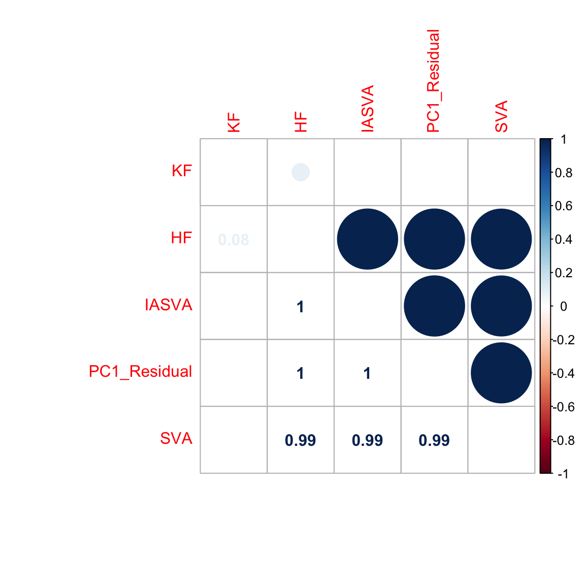
Several issues in the simulation studies suggested by the reviewer #2
We noticed several issues in these simulations. First, SVA or factor analysis based methods including IA-SVA are designed to estimate hidden variables with distinct levels (i.e., factors) or a transformation of factors. However, instead of simulating factors (e.g., a variable with two levels (1 and -1)) as typically done in such analyses1,2 (e.g., see http://jtleek.com/svaseq/simulateData.html and Method section (Simulated data) of https://www.biorxiv.org/content/biorxiv/early/2017/10/27/200345.full.pdf), the reviewer simulated numeric vectors from a uniform distribution (e.g., runif(1000)) and used them as hidden variables. We note that this leads, like IA-SVA, SVA also to perform poorly in the simulation study (r = -0.55) (see https://dleelab.github.io/iasvaExamples/reviewer2_sim.html). Second, IA-SVA does not accept intercept column in the design matrix; therefore instead of design, design[,-1] should have been used in these simulations. Third, the reviewer simulated counts using a Poisson distribution (mean = variance); however, negative binomial or zero-inflated negative binomial is a more appropriate model to simulate high variability (mean << variance) in bulk or single cell RNA-seq data. Fourth, even though only one hidden factor is simulated in the study, IA-SVA was forced to generate five hidden factors by setting the option ‘num.sv’ = 5. This leads IA-SVA to generate SV2-SV5, which are highly correlated SV1. To avoid this, we recommend users using the permutation procedure (by setting the default setting for option ‘permute’ (i.e, permute = TRUE) in ‘iasva’ function) or ‘fast_iasva’ function to determine the number of meaningful hidden factors. Lastly, to simulate a hidden factor with stronger effect sizes, the standard deviation (sd) in “unknown.effect <- rnorm(ngenes, sd=2)” should be increased (e.g., sd=4); rather increasing the range of simulated factor values from “unknown <- runif(1000, 0, 0.1)” to “unknown <- runif(1000)”. We have repeated the simulation studies by taking into consideration these points below.

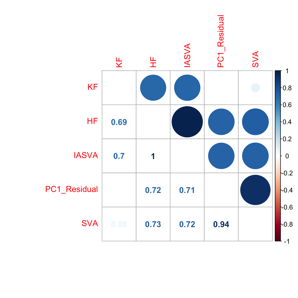
More challenging scenario.
Here, we simulated the known and hidden factors to affect only 100 (5%) and 20 (1%) genes respectively. We simulated the 20 genes affected by the hidden factor to be also affected by the known factor. Similarly, the two factors are highly correlated (r=0.7).
# Setting up the known and unknown factors.
set.seed(10000)

# to reduce the computational burden, we reduced the sample size (# of cells) and # of genes.
sample.size <- 100
ngenes <- 2000

# CORRECTEION: Here, we simulate factors with two levels (-1 or 1).
factor.prop <- 0.5
flip.prob <- 0.8 # to simulate high correlation btw known and hidden factors
known <- c(rep(-1,each=sample.size*factor.prop),rep(1,each=sample.size-(sample.size*factor.prop)))
coinflip = rbinom(sample.size,size=1,prob=flip.prob)
unknown = known*coinflip + -known*(1-coinflip)
cor(known, unknown) # correlation between known and unknown factors = 0.7
# [1] 0.6940221

# Generating Poisson count data from log-normal means.
# CORRECTION: to make factor with stronger effect size, we use 2 as SD here.
known.effect <- rnorm(ngenes, sd=2)
unknown.effect <- rnorm(ngenes, sd=2)

# To make estimation of the hidden factor more challenging, here we select 1900 (95%) and 1980 (1%) genes from each effect size vector and set their effect sizes as 0. That is, 5% and 1% of genes are affected by the known and hidden factors, respectively. All 20 genes affected by the hidden factor are affected by the known factor.

known.effect[1:1900] <- 0
unknown.effect[1:1980] <- 0

mat <- outer(known.effect, known) + outer(unknown.effect, unknown) + 2 # to get decent-sized counts
counts <- matrix(rpois(length(mat), lambda=2^mat), nrow=ngenes)
se <- SummarizedExperiment(assays=counts)

# Running IA-SVA, version 0.99.3.
library(iasva)
design <- model.matrix(~known)

# CORRECTION: IASVA doesn't accept the constant term of design matrix, so we use design[,-1] instead of design
res <- iasva(se, as.matrix(design[,-1]), threads=8) # iasva detected only one hidden factor.
# IA-SVA running...
#
# SV 1 Detected!
#
# # of significant surrogate variables: 1
# fast_iasva used here.
res.fast <- fast_iasva(se, as.matrix(design[,-1]), pct.cutoff = 2)  # fast_iasva detected only one hidden factor.
# fast IA-SVA running...
#
# SV 1 Detected!
#
# # of obtained surrogate variables: 1

#plot(res$sv[,1], unknown)
abs(cor(res$sv[,1], unknown)) ## absolute value of cor(SV1, unknown factor) = 0.9995
# [1] 0.9831191
abs(cor(res$sv[,1], known))   ## absolute value of cor(SV1, known factor) close to 0.7.
# [1] 0.8073574

#plot(res.fast$sv[,1], unknown)
abs(cor(res.fast$sv[,1], unknown)) ## absolute value of cor(SV1, unknown factor) = 0.9995
# [1] 0.9831191
abs(cor(res.fast$sv[,1], known))   ## absolute value of cor(SV1, known factor) close to 0.7.
# [1] 0.8073574


# Compare to just naively taking the first PC of the residual matrix.
library(limma)
resid <- removeBatchEffect(log(assay(se)+1), covariates=known)
pr.out <- prcomp(t(resid), rank.=1)
#plot(pr.out$x[,1], unknown)
abs(cor(pr.out$x[,1], unknown)) # cor = 0.7
# [1] 0.7114086
abs(cor(pr.out$x[,1], known)) # close to zero.
# [1] 3.193674e-16


# Compare to SVA
library(sva)
mod1 <- model.matrix(~known)
mod0 <- cbind(mod1[,1])
sva.res = svaseq(counts,mod1,mod0)$sv
# Number of significant surrogate variables is:  1
# Iteration (out of 5 ):1  2  3  4  5
#plot(sva.res[,1], unknown)
abs(cor(sva.res[,1], unknown)) # cor = 0.7
# [1] 0.6006951
abs(cor(sva.res[,1], known)) # close to zero.
# [1] 0.09633978

hf.mat5 <- cbind(known, unknown, res$sv[,1], pr.out$x[,1], sva.res[,1])
colnames(hf.mat5) <- c("KF","HF","IASVA","PC1_Residual","SVA")
corrplot.mixed(abs(cor(hf.mat5)), tl.pos="lt")
Expand here to see past versions of sim_corrected_high_corr_challenging-1.png:
| Version | Author | Date |
|---|---|---|
| 5e29c04 | dleelab | 2018-08-22 |
#par(oma = c(0, 2, 2, 2))
pdf("output/FigureL2.pdf", width=6,height=9)
par(mfrow=c(3,2))
corrplot.mixed(abs(cor(hf.mat1)), tl.pos="lt")
corrplot.mixed(abs(cor(hf.mat2)), tl.pos="lt")
corrplot.mixed(abs(cor(hf.mat3)), tl.pos="lt")
corrplot.mixed(abs(cor(hf.mat4)), tl.pos="lt")
corrplot.mixed(abs(cor(hf.mat5)), tl.pos="lt")
dev.off()
# quartz_off_screen
#                 2
Session information
sessionInfo()
# R version 3.5.0 (2018-04-23)
# Platform: x86_64-apple-darwin15.6.0 (64-bit)
# Running under: macOS Sierra 10.12.6
#
# Matrix products: default
# BLAS: /Library/Frameworks/R.framework/Versions/3.5/Resources/lib/libRblas.0.dylib
# LAPACK: /Library/Frameworks/R.framework/Versions/3.5/Resources/lib/libRlapack.dylib
#
# locale:
# [1] en_US.UTF-8/en_US.UTF-8/en_US.UTF-8/C/en_US.UTF-8/en_US.UTF-8
#
# attached base packages:
# [1] parallel  stats4    stats     graphics  grDevices utils     datasets
# [8] methods   base
#
# other attached packages:
#  [1] limma_3.36.2                corrplot_0.84
#  [3] SummarizedExperiment_1.10.1 DelayedArray_0.6.1
#  [5] matrixStats_0.53.1          Biobase_2.40.0
#  [7] GenomicRanges_1.32.3        GenomeInfoDb_1.16.0
#  [9] IRanges_2.14.10             S4Vectors_0.18.3
# [11] BiocGenerics_0.26.0         sva_3.28.0
# [13] BiocParallel_1.14.2         genefilter_1.62.0
# [15] mgcv_1.8-23                 nlme_3.1-137
# [17] iasva_0.99.3                workflowr_1.0.1
# [19] rmarkdown_1.9
#
# loaded via a namespace (and not attached):
#  [1] splines_3.5.0          lattice_0.20-35        htmltools_0.3.6
#  [4] yaml_2.1.19            blob_1.1.1             XML_3.98-1.11
#  [7] survival_2.42-3        R.oo_1.22.0            DBI_1.0.0
# [10] R.utils_2.6.0          bit64_0.9-7            GenomeInfoDbData_1.1.0
# [13] stringr_1.3.1          zlibbioc_1.26.0        R.methodsS3_1.7.1
# [16] evaluate_0.10.1        memoise_1.1.0          knitr_1.20
# [19] irlba_2.3.2            AnnotationDbi_1.42.1   Rcpp_0.12.17
# [22] xtable_1.8-2           backports_1.1.2        annotate_1.58.0
# [25] XVector_0.20.0         bit_1.1-14             digest_0.6.15
# [28] stringi_1.2.2          grid_3.5.0             rprojroot_1.3-2
# [31] tools_3.5.0            bitops_1.0-6           magrittr_1.5
# [34] RCurl_1.95-4.10        RSQLite_2.1.1          cluster_2.0.7-1
# [37] whisker_0.3-2          Matrix_1.2-14          git2r_0.21.0
# [40] compiler_3.5.0
This reproducible R Markdown analysis was created with workflowr 1.0.1